Machine learning and Steem #5: Account classification - understanding and using Ensemble Methods + tweaking performance
Repository
https://github.com/scikit-learn/scikit-learn
What Will I Learn?
- Collect data from beem and SteemSQL
- Understand the idea behind Ensemble Methods
- Use Ensemble Methods
- Averaging Methods: Bagging, RandomForest
- Boosting Methods: AdaBoost, GradientTreeBoosting
- Compare Ensemble Methods performance
- Tweak performance
Requirements
- python
- intermediate knowledge of data science / machine learning
Tools:
It may look like a lot of libraries, but it's a standard python toolset for data analysis / machine learning.

Difficulty
- Advanced
Tutorial Contents
- Problem description
- Collecting data
- 3D visualization
- Idea behind Ensemble Methods
- Using Ensemble Methods
- Comparing performance
- Tweaking performance
- What's next?
Problem description
The purpose of this tutorial is to build the steem account classifier, that will be able to distinguish between:
- content creator
- scammer
- comment spammer
- bid-bot
It is possible that the number of classes will change in the final version. The classifier, which was created in the last part of this tutorial, achieved an accuracy around 96%. In this section, Ensemble Methods will be used to further improve this result. It is also important that the execution time is acceptable.
The final goal is to build an API and web interface that will allow any Steem user to use this classifier.
Collecting data
The data was downloaded in a similar way to the previous part of the tutorial. Currently, each class has 822 records. The script that retrieves all the data can be found here.
The data looks as follows:
                 name  followers  followings  ...    comments_with_link_ratio  posts_to_comments_ratio  class
0          fuadmaulana        198          24  ...                    0.000000                 0.000000      0
1               ltfbyz         58          31  ...                    0.000000                 0.000000      0
2             papanero        460         191  ...                    0.000000                 0.624113      0
3           pialejoana        356          10  ...                    0.704641                 0.046414      0
4           adarshagni        700          63  ...                    0.000000                 3.000000      0
5           pialejoana        356          10  ...                    0.704641                 0.046414      0
6      uniqueknowledge        226          81  ...                    0.000000                 0.000000      0
7       jesusdiazmaica        190           7  ...                    0.000000                 0.000000      0
8        playfulfoodie       3820         537  ...                    0.022099                 0.254144      0
9             wakjal12        152          38  ...                    0.000000                 0.000000      0
10           iamfusion        201          60  ...                    0.000000                 0.000000      0
11           naruitchi        570         483  ...                    0.000000                 0.000000      0
12     mugiwaranohaqqi        395          83  ...                    0.000000                65.000000      0
13            click3rs       3814        5003  ...                    0.000000                10.125000      0
14          harwalis05        369         139  ...                    0.000000                 3.400000      0
15           taufit333        438         527  ...                    0.000000                 0.000000      0
16               unnun        354         121  ...                    0.000000                 2.000000      0
17             schubes        492         111  ...                    0.083333                 0.916667      0
18        ahmetsaritas        287          51  ...                    0.000000                 0.000000      0
19    grecki-bazar-ewy        697         181  ...                    0.142336                 0.054745      0
20        arthurbishop        116          43  ...                    0.000000                 0.000000      0
21            jozef230        982         504  ...                    0.291045                 0.212687      0
22             redjepi       1391          34  ...                    0.083333                 4.000000      0
23         puneetgamer         74          24  ...                    0.000000                 0.000000      0
24              godwyn        446         311  ...                    0.000000                 0.000000      0
25          lexikon082       1561         238  ...                    0.113095                 0.351190      0
26        good-joinned        871         194  ...                    0.000000                 0.000000      0
27          jumpmaster        805         194  ...                    0.000000                 0.671642      0
28       cheapproperty        283           8  ...                    0.000000                 0.333333      0
29            webgrrrl        368          25  ...                    0.000000                 3.000000      0
...                ...        ...         ...  ...                         ...                      ...    ...
3D visualization of features
To understand the data we are dealing with, it is worth to visualize it. We will use the mplot3d library and the code below.
# create 3D scatter plot
# x, y, z - names of features
def scatter_plot_3d(d, x, y, z):
    fig = plt.figure(figsize=(7, 7))
    # create 3D axes
    ax = Axes3D(fig)
    # plot points, cmap is colormap
    ax.scatter(d[x], d[y], d[z], c=d['class'], cmap=plt.cm.Accent, edgecolor='k', s=80)
    # set labels of each axis
    ax.set_xlabel(x)
    ax.set_ylabel(y)
    ax.set_zlabel(z)
    # add legend to plot
    # color of each legend label coresponds to color of given class
    ax.legend([label(color(150, 210, 150)), label(color(247, 192, 135)),
               label(color(235, 8, 144)), label(color(102, 102, 102))],
              ['content-creator', 'scammer', 'comment-spammer', 'bid-bot'], numpoints = 1)
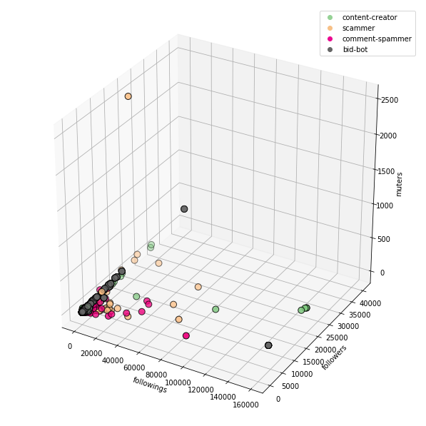
If we use raw data, the visualization may not be very readable, due to a number of values, which significantly differ from the whole dataset.
followings + followers + muters:
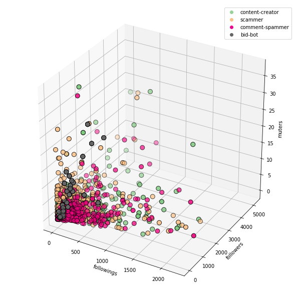
For this reason, it is worth to clean up the data that we will use for visualization. Just remove some of the outliers.
for column in columns:
    # calculate quantile (we want to remove 4% of the outliers)
    quantile = df[column].quantile(0.96)
    # filter column
    df1 = df1[df1[column] < quantile]
The charts are now much more readable.
followings + followers + muters:
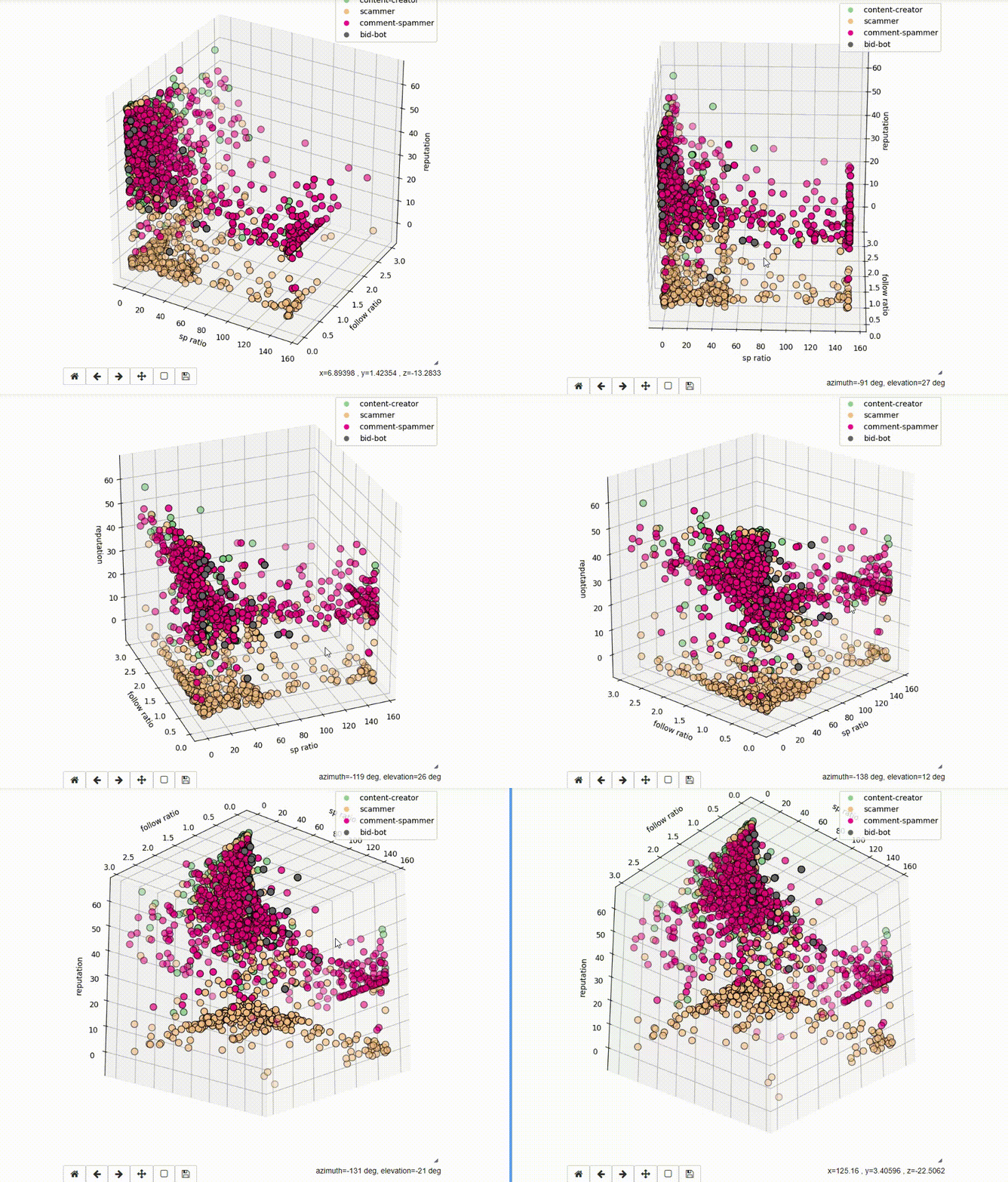
If we run the code as Jupyter Notebook, the charts are interactive.
Idea behind Ensemble Methods
Ensemble Methods can be divided into two groups:
- Averaging Methods
- Boosting Methods
The idea behind the Averaging Methods is to build several classifiers independently, and then use the weighted average as the final result. This usually leads to a better result, due to the reduced variance.
In the case of Boosting Methods it is different - we build classifiers sequentially, in order to minimize the bias of the combined estimator.
- Averaging Methods
- Bagging methods build several independent instances of a classifier on random subsets of the training dataset and then calculates final prediction from individual predictions. In this way, variance of the base classifier can be reduced.
- Random forests consists of trees built from a sample of the the training set. What's more, the split is the best split from a random subset of the features, not from all features.
- Extreme Random Trees are similiar to Random forests, but when performing a split, instead of looking for the most discriminating thresholds, the thresholds are chosen randomly for each candidate feature and the best of these randomly generated thresholds is selected.
- Boosting Methods
- AdaBoost aggregates sequence of weak estimators on modified versions of the training set. The final result is based on the vote of individual estimators.
- GradientTreeBoosting generalizes boosting to arbitrary differentiable loss functions
Using Ensemble Methods
The following code will be used to test the classifiers.
X_cols = columns
y_cols = ['class']
X = df[X_cols]
y = df[y_cols]
X_train, X_test, y_train, y_test = train_test_split(X, y, test_size=0.2, random_state=0)

# convert from pandas dataframe to plain array
y_train = np.array(y_train).ravel()
y_test = np.array(y_test).ravel()

# used classifiers: Decision tree for reference + ensemble methods
classifiers = [
    ('DecisionTreeClassifier', DecisionTreeClassifier(max_depth=8, random_state=0)),
    ('BaggingClassifier', BaggingClassifier(DecisionTreeClassifier(max_depth=8), max_samples=0.5, max_features=0.5)),
    ('RandomForestClassifier', RandomForestClassifier(max_depth = 10, n_estimators=10)),
    ('ExtraTreesClassifier', ExtraTreesClassifier(max_depth = 8, n_estimators=10, min_samples_split=2, random_state=0)),
    ('AdaBoost', AdaBoostClassifier(n_estimators=100)),
    ('GradientTreeBoosting', GradientBoostingClassifier(n_estimators=60, learning_rate=1.0, max_depth=1, random_state=0))
]

# iterate over classifiers
for clf_name, clf in classifiers:
    start = time.time()
    clf.fit(X_train, y_train)
    score = clf.fit(X_test, y_test)
    y_pred = clf.predict(X_test)
    end = time.time()
    print('%25s - accuracy: %.3f, execution time: %.3f ms' %
          (clf_name, accuracy_score(y_pred, y_test), end - start))
    cm = confusion_matrix(y_test, y_pred)
    plot_confusion_matrix(cm)
Compare Ensemble Methods performance
| Classifier | Acc | Time | Confusion matrix |
|---|---|---|---|
| DecisionTree | 0.945 | 0.026 | 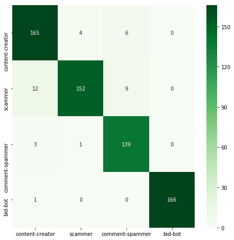 |
| Bagging | 0.941 | 0.069 | 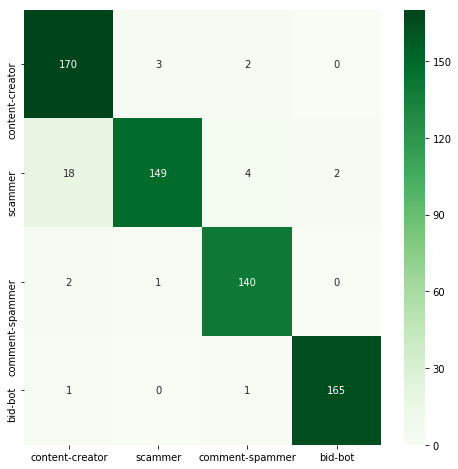 |
| RandomForest | 0.986 | 0.067 | 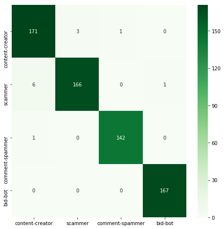 |
| ExtraTrees | 0.884 | 0.029 | 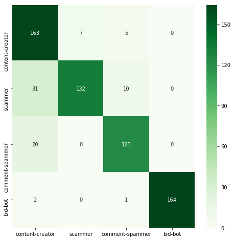 |
| AdaBoost | 0.767 | 0.617 | 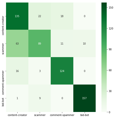 |
| GradientBoosting | 0.974 | 0.464 | 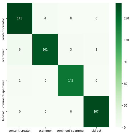 |
RandomForestClassifier and GradientBoostingClassifier achieved significantly better results than a single decision tree. AdaBoostClassifier turned out to be the worst classifier here, achieving accuracy far worse than all others. However, it's worth remembering that using ensemble methods often means increasing the execution time.
RandomForestClassifer consists of single trees, so we can visualize one of them with following code.
import graphviz
from sklearn.tree import export_graphviz

# convert decision tree metadata to graph
graph = graphviz.Source(export_graphviz(
    classifiers[2][1].estimators_[0], # select first decision tree from RandomForestClassifier
    out_file=None,
    feature_names=X_cols,
    class_names=class_names,
    filled=True,
    rounded=True))

# set format of output file
graph.format = 'png'
# save graph to file
graph.render('RandomForestClassifier')

Tweaking performance
RandomForestClassifier has achieved the best accuracy, which is why we will focus now on this classifier and try to improve this accuracy even more.
We will change the values of several parameters and check how it affected the result:
criterion- function which measures quality of split:giniorentropymin_samples_split- the minimum number of samples which is required to split a nodebootstrap- whether or not to use bootstrap samplesn_estimators- number of trees in the forestmax_depth- the maximum depth of the tree
The list of classifiers looks as follows.
classifiers = [
    ('RandomForestClassifier1', RandomForestClassifier(max_depth = 8, n_estimators=10, random_state=0)),
    ('RandomForestClassifier2', RandomForestClassifier(max_depth = 8, n_estimators=10, random_state=0, criterion='entropy')),
    ('RandomForestClassifier3', RandomForestClassifier(max_depth = 8, n_estimators=10, random_state=0, min_samples_split=2)),
    ('RandomForestClassifier4', RandomForestClassifier(max_depth = 8, n_estimators=10, random_state=0, bootstrap=True)),
    ('RandomForestClassifier5', RandomForestClassifier(max_depth = 8, n_estimators=100, random_state=0)),
    ('RandomForestClassifier6', RandomForestClassifier(max_depth = 10, n_estimators=100, random_state=0))
]
And here are the results.
   RandomForestClassifier1 - accuracy: 0.971, execution time: 0.065 ms
   RandomForestClassifier2 - accuracy: 0.976, execution time: 0.102 ms
   RandomForestClassifier3 - accuracy: 0.971, execution time: 0.061 ms
   RandomForestClassifier4 - accuracy: 0.971, execution time: 0.065 ms
   RandomForestClassifier5 - accuracy: 0.976, execution time: 0.603 ms
   RandomForestClassifier6 - accuracy: 0.992, execution time: 0.643 ms
Most parameters did not have a larger impact on the result. It was different in the case of max_depth, efficiency increased up to 99.2%. A further increase of this parameter keeps the result at a similar level. However, it must be remembered that too high depth may not be very beneficial because it increases the execution time and can lead to overfitting of the classifier.
Below is the confusion matrix for the best result.

What's next?
- building API for classifier
- building web interface for classifier
- enlarging the dataset
Curriculum
- Machine learning (Keras) and Steem #1: User vs bid-bot binary classification
- Machine learning and Steem #2: Multiclass classification (content creator vs scammer vs comment spammer vs bid-bot)
- Machine learning and Steem #3: Account classification - accuracy improvement up to 95%
- Machine learning and Steem #4: Account classification - comparison of available classifiers + 3D visualization of features
Conclusions
- it is worth to clean data before visualization to remove outliers
- 3D visualization allows you to show more information than 2D visualization, but on the other hand, the data can be less readable
- classifiers can be combined with each other in different ways
- combining classifiers can reduce bias or variance, so that the final accuracy can be better
- combining classifiers also means increasing the execution time, so you often have to choose between accuracy and execution time
- performance can be improved by changing parameters
Thank you for your contribution.
I loved the work you did here, and i remember earlier contributions of yours. You've been away for some time, don't .. we love your work :)
Overall excellent work, visualizations and different methodology descriptions are quite useful. Iterating a bit further on some concepts for the purpose of a tutorial might have been a bit more helpful to your readers.
Can't wait to see your final product and API. It seems Steem will now have a multitude of account classifications systems, which is definitely positive!
Your contribution has been evaluated according to Utopian policies and guidelines, as well as a predefined set of questions pertaining to the category.
To view those questions and the relevant answers related to your post, click here.
Need help? Write a ticket on https://support.utopian.io/.
Chat with us on Discord.
[utopian-moderator]
Thank you for your review, @mcfarhat! Keep up the good work!
Hello! Your post has been resteemed and upvoted by @ilovecoding because we love coding! Keep up good work! Consider upvoting this comment to support the @ilovecoding and increase your future rewards! ^_^ Steem On!

Reply !stop to disable the comment. Thanks!
Hi @jacekw.dev!
Your post was upvoted by @steem-ua, new Steem dApp, using UserAuthority for algorithmic post curation!
Your post is eligible for our upvote, thanks to our collaboration with @utopian-io!
Feel free to join our @steem-ua Discord server
Congratulations @jacekw.dev! You have completed the following achievement on the Steem blockchain and have been rewarded with new badge(s) :
Click here to view your Board of Honor
If you no longer want to receive notifications, reply to this comment with the word
STOPDo not miss the last post from @steemitboard:
Hey, @jacekw.dev!
Thanks for contributing on Utopian.
Congratulations! Your contribution was Staff Picked to receive a maximum vote for the tutorials category on Utopian for being of significant value to the project and the open source community.
We’re already looking forward to your next contribution!
Get higher incentives and support Utopian.io!
Simply set @utopian.pay as a 5% (or higher) payout beneficiary on your contribution post (via SteemPlus or Steeditor).
Want to chat? Join us on Discord https://discord.gg/h52nFrV.
Vote for Utopian Witness!
Ja cie krece, nie wiedzialem ze masz drugie konto :) solidne tutoriale, szanuje.
Congratulations @jacekw.dev! You have completed the following achievement on the Steem blockchain and have been rewarded with new badge(s) :
Click here to view your Board of Honor
If you no longer want to receive notifications, reply to this comment with the word
STOPDo not miss the last post from @steemitboard: