Putting it all together - Introduction to Tensorflow Part 5

This is the last part of a multi part series. If you haven't already, you should read the previous parts first.
- Part 1 where we discussed the design philosophy of Tensorflow.
- Part 2 where we discussed how to do basic computations with Tensorflow.
- Part 3 where we discussed doing computations at a scale (GPUs and multiple computers) as well as how we can save our results.
- Part 4 where we learned how to make visualizations with Tensorflow.
This time we will wrap up everything we learned in a real world example: creating a small neural network.
This post originally appeared on kasperfred.com where I write more about machine learning.
An almost practical example
While the small examples up until now are great at demonstrating individual ideas, they do a poor job of showing how it all comes together.
To illustrate this, we will now use everything (well, almost everything) we have learned about Tensorflow to make something we at least can pretend to be somewhat practical; we will build a very simple neural network to classify digits from the classic MNIST dataset. If you're not fully up to speed with neural networks, you can read this introduction (coming soon) before coming back to this.
The construction and training of the neural network can be broken down into a couple of phases:
- Importing the data.
- Constructing the model architecture.
- Defining a loss function to optimize, and a way to optimize it.
- Actually training the model.
- Evaluating the model.
However, before we can start creating the model, we must first prepare Tensorflow:
import tensorflow as tf
tf.reset_default_graph() # again, this is not needed if run as a script
Next, we import the data.
from tensorflow.examples.tutorials.mnist import input_data
mnist = input_data.read_data_sets("MNIST_data/", one_hot=True)
Extracting MNIST_data/train-images-idx3-ubyte.gz
Extracting MNIST_data/train-labels-idx1-ubyte.gz
Extracting MNIST_data/t10k-images-idx3-ubyte.gz
Extracting MNIST_data/t10k-labels-idx1-ubyte.gz
Since mnist is such a well known dataset, we can use the built in data extractor to get a nice wrapper around the data.
Now, it's time to define the actual model that's going to be used. For this task, we will use a feed forward network with two hidden layers that has 500 and 100 parameters respectively.
Using the idea about scopes to separate the graph into chunks, we can implement the model like so:
# input
with tf.name_scope('input') as scope:
    x = tf.placeholder(tf.float32, [None, 28*28], name="input")
    # a placeholder to hold the correct answer during training
    labels = tf.placeholder(tf.float32, [None, 10], name="label")
    # the probability of a neuron being kept during dropout
    keep_prob = tf.placeholder(tf.float32, name="keep_prob")

with tf.name_scope('model') as scope:
    with tf.name_scope('fc1') as scope: # fc1 stands for 1st fully connected layer
        # 1st layer goes from 784 neurons (input) to 500 in the first hidden layer
        w1 = tf.Variable(tf.truncated_normal([28*28, 500], stddev=0.1), name="weights")
        b1 = tf.Variable(tf.constant(0.1, shape=[500]), name="biases")

        with tf.name_scope('softmax_activation') as scope:
            # softmax activation
            a1 = tf.nn.softmax(tf.matmul(x, w1) + b1)

        with tf.name_scope('dropout') as scope:
            # dropout
            drop1 = tf.nn.dropout(a1, keep_prob)

    with tf.name_scope('fc2') as scope:
        # takes the first hidden layer of 500 neurons to 100 (second hidden layer)
        w2 = tf.Variable(tf.truncated_normal([500, 100], stddev=0.1), name="weights")
        b2 = tf.Variable(tf.constant(0.1, shape=[100]), name="biases")

        with tf.name_scope('relu_activation') as scope:
            # relu activation, and dropout for second hidden layer
            a2 = tf.nn.relu(tf.matmul(drop1, w2) + b2)

        with tf.name_scope('dropout') as scope:
            drop2 = tf.nn.dropout(a2, keep_prob)

    with tf.name_scope('fc3') as scope:
        # takes the second hidden layer of 100 neurons to 10 (which is the output)
        w3 = tf.Variable(tf.truncated_normal([100, 10], stddev=0.1), name="weights")
        b3 = tf.Variable(tf.constant(0.1, shape=[10]), name="biases")

        with tf.name_scope('logits') as scope:
            # final layer doesn't have dropout
            logits = tf.matmul(drop2, w3) + b3
For training, we are going to use the cross entropy loss function together with tha ADAM optimizer with a learning rate of 0.001. Following the example above, we continue the use of scopes to organize the graph.
We also add two summarizers for accuracy and the average loss, and create a merged summary operation to simplify later steps.
Finally, once we add the saver object, so we don't lose the model after training (which would be a shame), we have this:
with tf.name_scope('train') as scope:
    with tf.name_scope('loss') as scope:
        # loss function
        cross_entropy = tf.nn.softmax_cross_entropy_with_logits(labels=labels, logits=logits)
    # use adam optimizer for training with a learning rate of 0.001
    train_step = tf.train.AdamOptimizer(0.001).minimize(cross_entropy)

with tf.name_scope('evaluation') as scope:
    # evaluation
    correct_prediction = tf.equal(tf.argmax(logits,1), tf.argmax(labels,1))
    accuracy = tf.reduce_mean(tf.cast(correct_prediction, tf.float32))

# create a summarizer that summarizes loss and accuracy
tf.summary.scalar("Accuracy", accuracy)

# add average loss summary over entire batch
tf.summary.scalar("Loss", tf.reduce_mean(cross_entropy))

# merge summaries
summary_op = tf.summary.merge_all()

# create saver object
saver = tf.train.Saver()
It's now time to begin training the network. Using the techniques discussed previously, we write a summary every 100 steps for the total of 20000 steps.
At each step we train the network with a batch of 100 examples by running the train_step operation which will update the weights of network in accordance with the learning rate.
Finally, once the learning is done, we print out the test accuracy, and save the model.
with tf.Session() as sess:
    # initialize variables
    tf.global_variables_initializer().run()

    # initialize summarizer filewriter
    fw = tf.summary.FileWriter("/tmp/nn/summary", sess.graph)

    # train the network
    for step in range(20000):
        batch_xs, batch_ys = mnist.train.next_batch(100)
        sess.run(train_step, feed_dict={x: batch_xs, labels: batch_ys, keep_prob:0.2})

        if step%1000 == 0:
            acc = sess.run(accuracy, feed_dict={
                x: batch_xs, labels: batch_ys, keep_prob:1})
            print("mid train accuracy:", acc, "at step:", step)

        if step%100 == 0:
            # compute summary using test data every 100 steps
            summary = sess.run(summary_op, feed_dict={
                x: mnist.test.images, labels: mnist.test.labels, keep_prob:1})

            # add merged summaries to filewriter,
            # so they are saved to disk
            fw.add_summary(summary, step)

    print ("Final Test Accuracy:", sess.run(accuracy, feed_dict={
                x: mnist.test.images, labels: mnist.test.labels, keep_prob:1}))

    # save trained model
    saver.save(sess, "/tmp/nn/my_nn.ckpt")
mid train accuracy: 0.1 at step: 0
mid train accuracy: 0.91 at step: 1000
mid train accuracy: 0.89 at step: 2000
mid train accuracy: 0.91 at step: 3000
[...]
mid train accuracy: 0.97 at step: 17000
mid train accuracy: 0.98 at step: 18000
mid train accuracy: 0.97 at step: 19000
Final Test Accuracy: 0.9613
96% accuracy is that any good?
No, that actually kind of sucks, but the point of this network is not to be the best network. Instead, the point of it is to demonstrate how you can use Tensorflow to construct a network, and get a lot of visualization pizzazz for very little work.
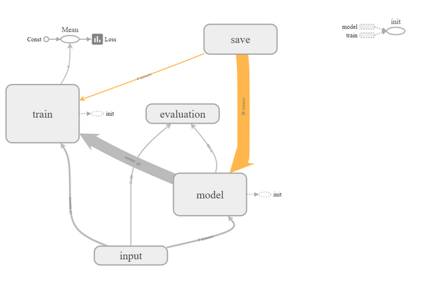
If we run the model, and open it in tensorboard, we get:

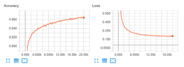
Furthermore, we can see the summaries Tensorflow made for the accuracy and loss, and that they do, as expected, behave approximately like inverse of each other. We also see that the accuracy increases a lot in the beginning, but flattens out over time which is expected partly because we use the ADAM optimizer, and partly because the nature of gradients.

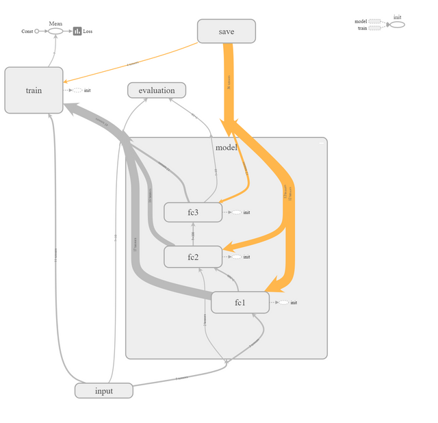
The use of nested scopes let's us progressively change the abstraction level. Notice how, if we expand the model, we can see the individual layers before the individual layer components.

If you want to run this network yourself, you can access the code on Github.
Conclusion
Wow, you're still here. You deserve a cute picture of a cat.

If you have followed this far, you should now be comfortable with the basics of Tensorflow: How it functions, how to do basic computations, how to visualize the graph, and finally you have seen a real example of how it can be used to create a basic neural network.
Also, send me a tweet @kasperfredn if you made it all the way through: You're awesome.
As this was just an introduction to Tensorflow, there's a lot we didn't cover, but you should know enough now to be able to understand the API documentation where you can find modules you can incorporate into your code.
If you want a challenge to test your comprehension, try to use Tensorflow to implement another machine learning model by either working from the model we created here, or starting from scratch.
Congratulations @kasperfred! You have completed some achievement on Steemit and have been rewarded with new badge(s) :
Click on any badge to view your own Board of Honor on SteemitBoard.
For more information about SteemitBoard, click here
If you no longer want to receive notifications, reply to this comment with the word
STOP