Using harmonic modulation for N=1 experiments (Part 2/3)

Using harmonic modulation for N=1 experiments (Part 2/3)

This is the second post in this series about the use of harmonically simulated input variables in N=1 experiments. In my previous post in this series, we covered an intro into black box analysis using harmonic inputs to establish just the existence of a transposition from the harmonic input signal to an output. We did this with a very noisy black box with some harmonic output frequencies that were present regardless of our input. In a situation as noisy as the one discussed in our first post, this would be as far as we could get.

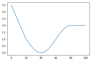
In this post, we look at a little bit less noisy black box and see how much further it could get us. Let's start off by revisiting our transpositional function.

%matplotlib inline
import math
import numpy as np
import matplotlib.pyplot as plt
from scipy.fftpack import fft

def transpose(x):
    if x < 20:
        return 3.5 - x/8
    if x > 80:
        return 2
    return 1 - math.sin((x-20)*math.pi/40)

x = np.linspace(0,100,num=100)
y = np.array([transpose(xi) for xi in x])
plt.plot(x, y)

[<matplotlib.lines.Line2D at 0x7f55c0923978>]

Now let us use a less aggresive version of our prevous complex_transpose function. No internal harmonics, just two sources of internal noice.

def complex_transpose(x):
    input_noice = np.random.normal(0, 10, size=1)[0]
    internal_x = x + input_noice
    internal_y = transpose(internal_x)
    output_noice = np.random.normal(0, 0.5, size=1)[0]
    rval = internal_y + output_noice
    if rval < 0:
        return 0
    else:
        return rval

x = np.linspace(0,100,num=100)
y = np.array([complex_transpose(xi) for xi in x])
plt.plot(x, y)
    
    

[<matplotlib.lines.Line2D at 0x7f55c0764630>]

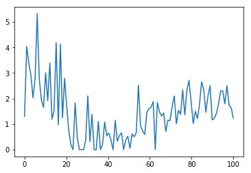
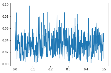
The noice level is much lower, and we see some traces of our original transposition function, but only because we know what to look for. Let's look at the fourier transform of the noice for a static input of 50:

x = np.linspace(0,1000,num=1000)
y = np.array([complex_transpose(50) for xi in x])

N = len(y)
T = 1
yf = fft(y)
absyf = 2.0/N * np.abs(yf[0:N//2])
xf = np.linspace(0.0, 1.0/(2.0*T), N//2)
plt.plot(xf[1:], absyf[1:])

[<matplotlib.lines.Line2D at 0x7f55c066df60>]

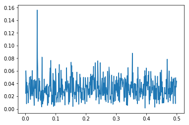
Let add in our harmonic signal

def harmonic_transpose(t,x,amplitude,harmonic):
    h = amplitude * math.sin(harmonic * t * 2 * math.pi)   
    return complex_transpose(x + h)

t = np.linspace(0,1000,num=1000)
y = np.array([harmonic_transpose(ti,50,5,5/127) for ti in t])
N = len(y)
T = 1
yf = fft(y)
absyf = 2.0/N * np.abs(yf[0:N//2])
xf = np.linspace(0.0, 1.0/(2.0*T), N//2)
plt.plot(xf[1:], absyf[1:])
print(5/127)
    

0.03937007874015748

Or zoomed in into our own harmonic:

plt.plot(xf[30:60], absyf[30:60])

[<matplotlib.lines.Line2D at 0x7f55c3062780>]

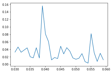
As you probably noticed, we used a rather low amplitude this time. We are doing this for a reason. We are going to sample the hidden transposition function by modulating different input signal base levels with our low amplitude harmonic signal. This is the part where for our N=1 situation things will get hard. More about that in the final instalment from this series. For now, lets look how we can sample the transposition function.

def closest_value(harmonic, xf, yf, absy,x):
    best_index = 0
    best_match = abs(xf[0] - harmonic)
    for index in range(1,len(xf)):
        if abs(xf[index] - harmonic) < best_match:
            best_index = index
            best_match = abs(xf[index] - harmonic)
    return x,round(absy[best_index],2),round(np.angle(yf[best_index], deg=True),1)

res = closest_value(5/127,xf,yf,absyf,50)
print(res)

(50, 0.16, -24.8)

Let us do this for sample level 10,20,30,40,50,60,70,80 and 90 ans see what we get.

def get_transposition_meta(x,amplitude,harmonic):
    t = np.linspace(0,1000,num=1000)
    y = np.array([harmonic_transpose(ti,x,amplitude,harmonic) for ti in t])
    yf = fft(y)
    N = len(y)
    T = 1
    xf = np.linspace(0.0, 1.0/(2.0*T), N//2)
    abs_yf = 2.0/N * np.abs(yf[0:N//2])
    return closest_value(harmonic, xf, yf, abs_yf,x)

meta = np.array([get_transposition_meta(ctr,5,5/127) for ctr in [10,20,30,40,50,60,70,80,90]])
meta

array([[ 1.000e+01,  3.600e-01,  1.561e+02],
       [ 2.000e+01,  2.900e-01,  1.705e+02],
       [ 3.000e+01,  1.600e-01,  1.768e+02],
       [ 4.000e+01,  6.000e-02,  1.150e+01],
       [ 5.000e+01,  1.500e-01, -1.210e+01],
       [ 6.000e+01,  2.500e-01, -1.810e+01],
       [ 7.000e+01,  1.600e-01, -2.050e+01],
       [ 8.000e+01,  9.000e-02, -1.120e+01],
       [ 9.000e+01,  3.000e-02, -7.030e+01]])

Now we have a bit of a problem that we haven't been addressing that you might have spotted. If we look again at our frequency spectrum, we see a lot of peeks that are just noice. Only one of them isn't, that is, only one of then isn't just noice. As this one is the one we will be looking at in detail next, the noice part of the peek we are interested in might very well show us stuff that isn't really there. We could pull out the math and the statistics here, but lets not do this now as to keep this hands on. Just look at our frequency spectrum and pick the five highest peeks, appart from the one we created ourselves, We could draw a line at about 0.75 and capture all but these five outliers. The chances of such an outlier hitting exactly our frequency are slim but not zero. If it ended up hitting us, we would want its impact to not make our findings complete nonsense.

We could pick an optimistic treshold at about twice this value, or go for a much more conservative one and choose three times this value. Let us choose the optimistic route and set our treshold at 0.15.

meta[np.where(meta[:,1] > 0.15)]

array([[ 1.000e+01,  3.600e-01,  1.561e+02],
       [ 2.000e+01,  2.900e-01,  1.705e+02],
       [ 3.000e+01,  1.600e-01,  1.768e+02],
       [ 6.000e+01,  2.500e-01, -1.810e+01],
       [ 7.000e+01,  1.600e-01, -2.050e+01]])

So now we are left with modulation points at 10,20,30,60 and 70. The modelation points at 40,50 80 and 90 are ignored as they are simply too likely to yield nonsensical results. Now it is time to focus on the third column of our little matrix, the angle. Remember, there are 360 degrees on a circle. Let us not get distracted by the minus signs and focus on two numbers. The first three numbers are relatively close. With a mean value of 167.8. The other two numbers are also close with a mean value of -19.5. The difference between the two means is 187.3. This is important because 180 degrees is an important number. 180 degrees means an inversion in the direction of the transposition function. If we assume there are no intrinsic delays in our black box, then an angle close to zero degrees means that an increase in the input leads to an increase in the output, and if the angle is close to 180 degrees, an increase in the input leads to a decrease in the output.

It is essential to realize that a system intrincic delay that goes unrecognized could lead to wrong conclusions. Repeating the experiment at different harmonic frequencies can be used to tease out the pressence and the size of system intrinsic delays. This subject however flls outside of the scope of this primer. For now, we assume we know the system has no intrincic delays and the numbers we got can give us usefull info.

If we take the two values in our filtered outcomes together, we can now write the info a bit differently to make it more clear what we have found so far:

• At an input value of 10, we have a slope of about -0.36 c (where c is an unknown constant)
• At an input value of 20, we have a slope of about -0.29 c
• At an input value of 30, we have a slope of about -0.16 c
• Somewhere above 30 but below 60 we have a local minimum (or possibly maximum if we expected delays)
• At an input value of 60, we have a slope of about 0.25 c
• At an input value of 70, we have a slope of about 0.16 c
• The slope above 70 is to weak to extract any reliable info.

Now have an other look at our initial image on this page and see how things fit. Notice how much valuable information we were able to extract despite of the noicyness of the system?

In reality, you wont always be as lucky to reconstruct this much information in your N=1 experiments, as we shall see in the last instalment of this series. There are constraints and difficulties in applying this theory to a situation where the input might be the amount of coffee consumed and the output might be something like a specific marker from a at-home urine test. These constraints or dificulties might be time bound, of a financial nature, or simply due to the need for accuracy and disipline that might require a personality with traits bordering on OCD.

Personaly I feel that despite of the constraints and dificulties, no one doing N=1 experiments with his diet and workout routeen will be able to get the best out of his experiments without at least considering harmonic input modellation blackbox analysis techniques like the ones described in this primer.