SEC | S20W2 | Data Analysis with Google Sheets: (Advanced Excel formulas, and pivot tables.)
 source source |
|---|
Hello Everyone!!
It's good to be here, learning they say never ends and I totally believe it. So far the lecture has been interesting and here I bring my home work answers to you.
Explain what you understand by Advanced Excel Formulas, and show us where advanced formulas such as the lookup function, and logical function are found in Excel with clear screenshots |
|---|
Advanced excel formulas are generally described as commands or functions that can be used to carryout out complex task such as calculations, creating reports, analyzing data and creating dashboards.
These functions or commands are usually found in the Excel. Meaning they are built together with the excel.
Sometimes, some of these advanced excel formulas can be used alone or can be combined with other advanced formulas to carry out the assigned task.
Examples of advanced excel formulas are SUMIF, LOOKUP, INDEX and many others.
Steps to show where lookup functions and logical function are located
- I open my spreadsheet on my phone.
- I click on a column on the spreadsheet
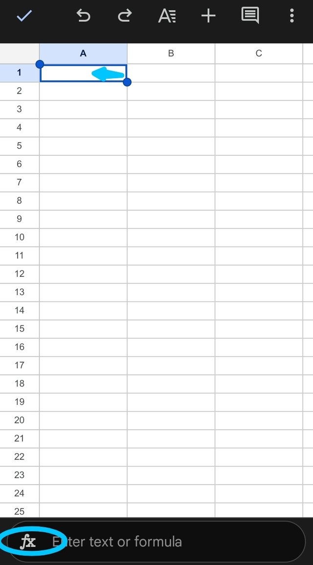
- Downwards I located the text bar and clicked on the formula icon fx as seen on the screenshot below
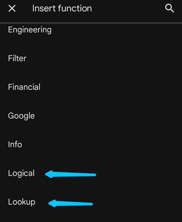
- The insert function opens up
- There I found the lookup function and the logical function.
 |  |
|---|
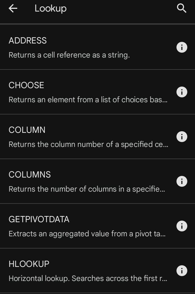
- Next I clicked on the lookup function and it brings out other functions under it. As seen. In the screenshot below.
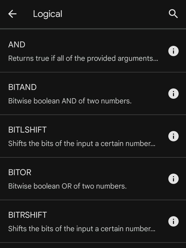
- I also clicked on the logical function to check through. As seen in the screenshot below.
 |  |
|---|
Write the IF Function formula to calculate the total, average score, and grade of students given in the table below |
|---|
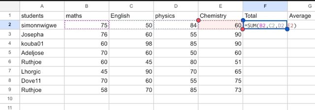
To calculate Total of the student I used the formula =SUM(B2,C2,D2,E2) because the IF function can not be used to calculate Total as seen in screenshot 1 and 2 below
 1 1 |  2 2 |
|---|
To calculate the average of students I used the IF formula =AVERAGE(B2,C2,D2,E2) as seen in the screenshot 3 and 4, because the IF formula can not be used to calculate the average of the student.
 3 3 |  4 4 |
|---|
To calculate the grades of students I used the the formula =IF(G2>=70, "A", IF(G2>=60, "B", IF(G2>=50, "C", IF(G2>=45, "D", IF(G2>=40, "E", "F"))))) as seen in screenshot 5 and 6
 5 5 |  6 6 |
|---|
Based on the given data below: Create a pivot table that shows (see) total sales by product, by dragging the product to the Rows areas, Region to the Column area, and Sales to the Values area. Please we want to see the steps you take in adding your pivot table |
|---|
Am creating a pivot table using my mobile phone.
The first step is to open my spreadsheet on my phone.
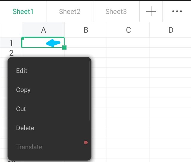
When it opens,Click on a column as seen in screenshot 1 below.
When I click on the column, I locate edit so that I can type in the column as seen in screenshot 2 below.
 1 1 | 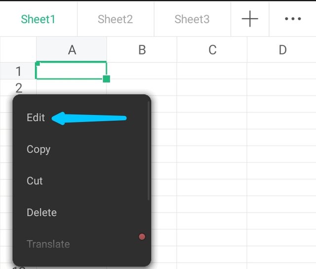 2 2 |
|---|
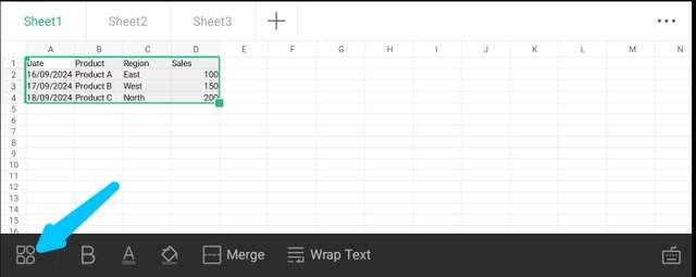
I followed the same procedure until I was done typing in all my items on coloums and rows from date, Product ,region and sales. As seen in the screenshot below.

Next I highlight the whole item I have typed and clicked on the icon at the tool bar as seen in the screenshot below.
When it opens I clicked on the insert option I circled on my screenshot below, then I scrolled to located the pivot table and clicked it. See the screenshot below.
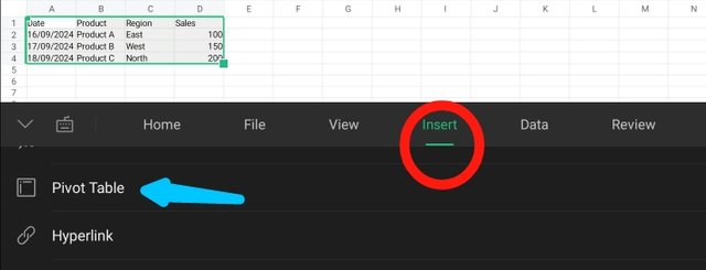
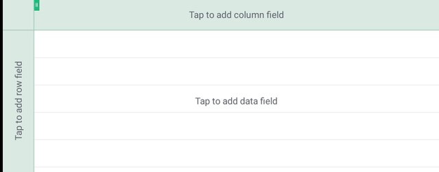
When I clicked on the pivot table, it inserted on another spreadsheet sheet because am using a phone. As seen on the screenshot A below
Next I clicked on the column field to add the region and I clicked on the row field to add the product ans finally the data field to add sales value. Check the screenshot B below.
 A A | 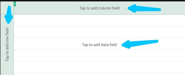 B B |
|---|
Once I completed filling in all my data what I have is the screenshot below.
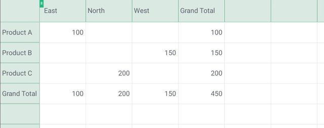
Thank you so much for the lessons, it was not easy using the mobile phone for this home work. I think a laptop is much easier. Soon I would be able to afford the means to get a laptop.
I would like to invite some friends to join this contest @ninapenda @jovita30 @hisgeneral
Upvoted. Thank You for sending some of your rewards to @null. It will make Steem stronger.
Your post has been rewarded by the Seven Team.
Support partner witnesses
We are the hope!
Congratulations! Your post has been upvoted through steemcurator06.

Good post here should be . . .
Curated by : @𝗁𝖾𝗋𝗂𝖺𝖽𝗂
Thank you so much @heriadi
This post has been upvoted/supported by Team 7 via @httr4life. Our team supports content that adds to the community.