SEC | S20W2 | Data Analysis with Google Sheets: (Advanced Excel formulas, and pivot tables.)
Hello steemians of all denomination. Greetings to you all and welcome to this week's engagement challenge. I am so delighted to be participating on this amazing topic on excell brought to us by a wonderful team. Making it brief, I will begin with the discussion on here right away.
Data analysis is the arrangement of specific information in a particular way which is more appealing and informative to the taste of the person in question. This could be done with the use of Excel, libre office or Google sheets. Other third party Applications can be used for this too.
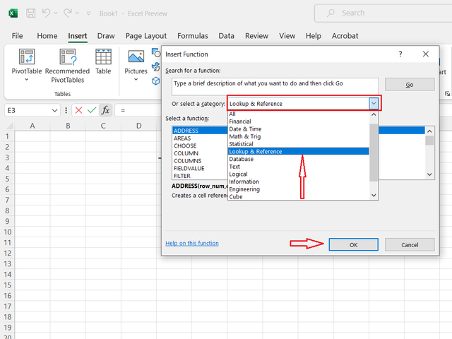
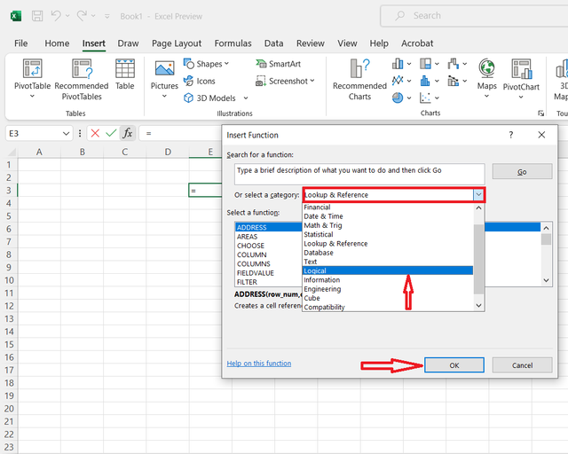
Explain the understanding of Advanced Excel Formulas, and show details where advanced formulas such as the lookup function, and logical function are found in Excel with clear screenshots.
Understanding Advanced Excel Formulas
Advanced Excel formulas are powerful tools that can help you perform complex calculations, manipulate data, and automate tasks. They go beyond the basic arithmetic operations and allow you to work with more intricate datasets.
Lookup Functions
Lookup functions are used to find specific values within a table or range of cells based on a given criteria.
VLOOKUP: commonly known as vertical look up, these looks up indicates a value in the leftmost column of a given table and will returns a corresponding value from the same row.
HLOOKUP: By name Horizontal look up. The look up indicates a value in the top row of a table and will returns a corresponding value from the same column.
INDEX-MATCH: A combine
INDEXandMATCHfunctions that generate more flexibility thanVLOOKUPandHLOOKUP,allowing you to look up values in any part of a any given table.
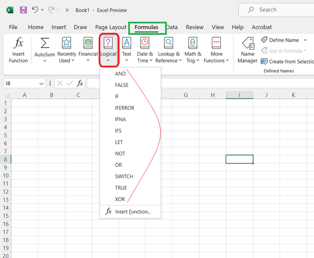
Logical Functions.
Logical functions are implemented to perform logical tests and return values based on the results of these tests in question.
IF:Used to where we have to Returns one value incase a condition is true, and another value if it's false.
We have.<, >, >=,<=, <>
Finding Advanced Formulas in Excel:
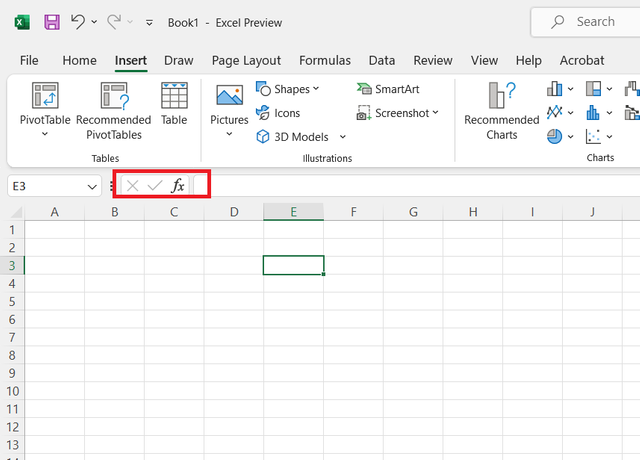
Insert Function:
- Navigate to
"fx"icon in the formula bar.
- Navigate to
- Search for the desired function in the
"Insert Function"dialog box.
 |  |
|---|
Formula Bar:
- Begin by typing the name of the function in the formula bar. A list of matching functions will drop down. You click on the desire formula.
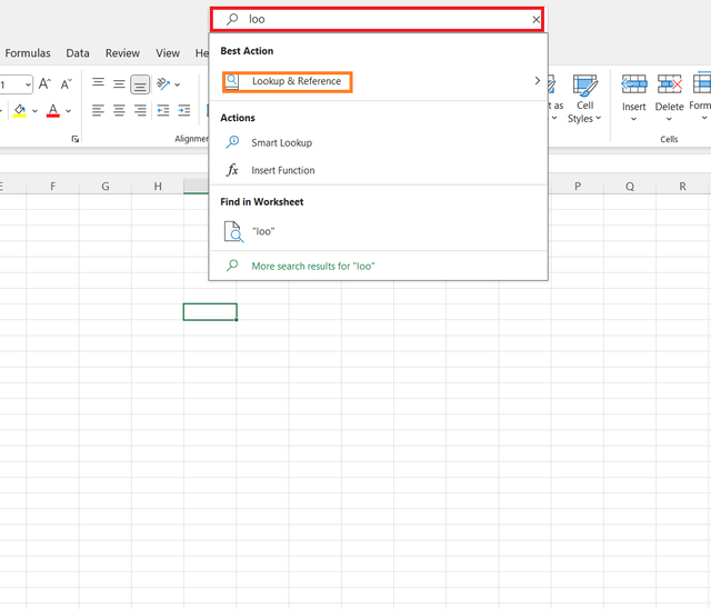
- Begin by typing the name of the function in the formula bar. A list of matching functions will drop down. You click on the desire formula.
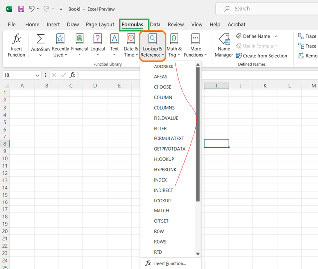
Function Library:
- Go to the
"Formulas"tab and click on the "Insert Function" button to access the function library.
- Go to the
 |  |
|---|
Write the IF Function formula to calculate the total, average score, and grade of students given in the table below._____
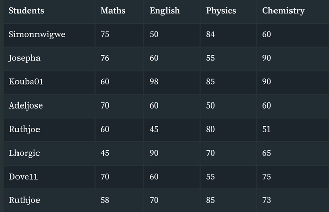
To begin with, we are going to fill in the marks by recreating the table above.
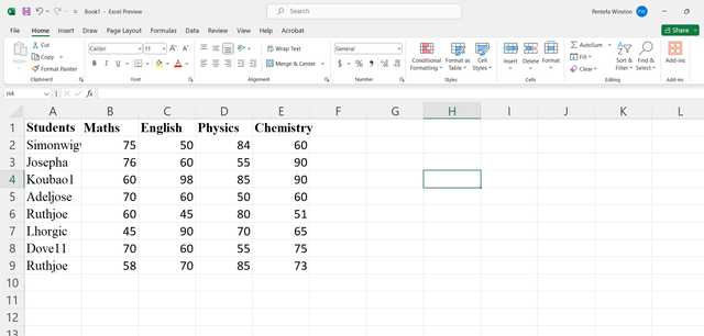
Next step we proceed to add the cells for the total average and Grade of these students.
For these cells we will employ the following formulas
=Sum(B2:D2)and then drag down to fill the rest of the columns automatically.
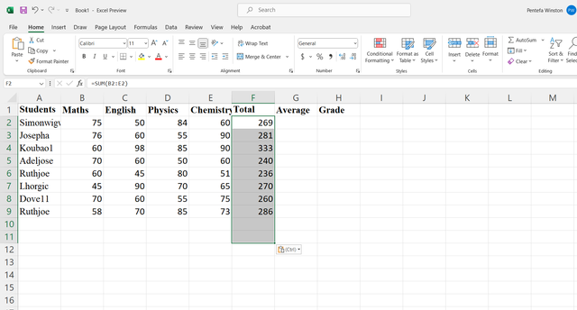
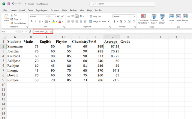
For average function we will you the formula for average. We have indicated in the above writing 3 places to get get these formulas.
- Input
=Average (B2:D2)and then hit enter. This gives the first point and we drag down to fill the remaining spaces.
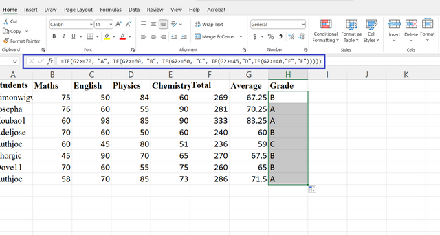
For the grade let get to you the logical function IF. to begin with, we input the formula. =IF(G2>=70, "A", IF(G2>=60, "B", IF(G2>=50, "C", IF(G2>=45, "D", IF(G2>=40, "E", "F")))))
Briefly discuss four IF function Operators that I have learned and tell their functions and when we are to use them_____
So far , we have learned IF functions like >,< , =, <=, >=, <>,
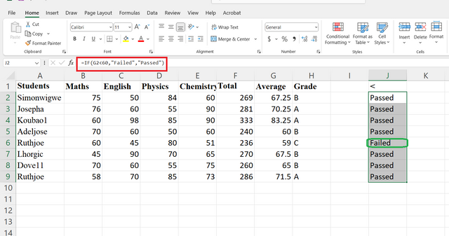
1• Using <:
This just logical function is used In case where we are making a judgment about A variable in a particular limit for instance, any number less than 60 Should be assigned as failed while any number above 60 should be assigned a passed. This is possible by using the logical function =IF(G2<60,"FAILED","PASSED")
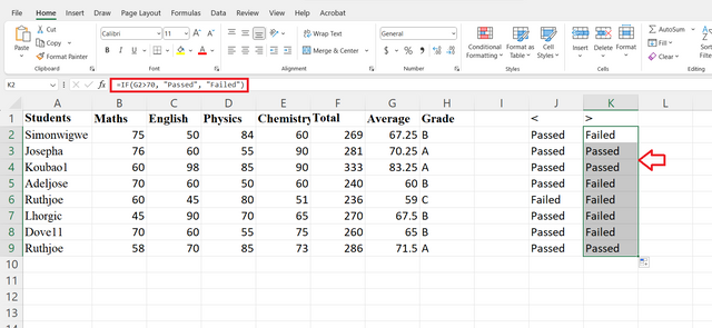
2• Using the > function.
This is used in the same way at the less than function, but the difference is we are going to assign our true value to be a passed and our false value to be a failed. We do this by implementing =IF(G2>70,"PASSED","FAILED")
3• Using <=function.
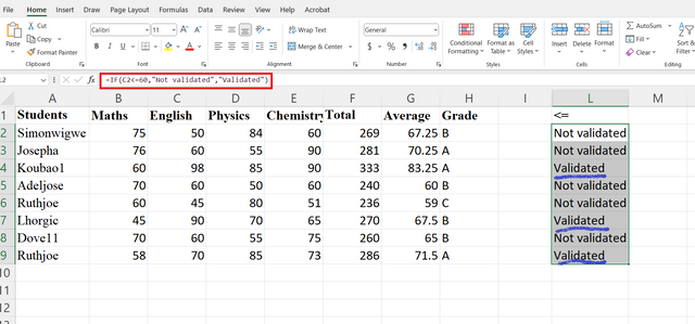
This function Is read as less than or equal to. To apply it, we are about to compare a verb based on a certain limit and above. For instance we can say any number From 60 and above to assign as validated and any number below 60 and above should be assigned not validated
We are going to employ the formula. =IF(C2<=60, "not validated", "validated")
4• using the >=function
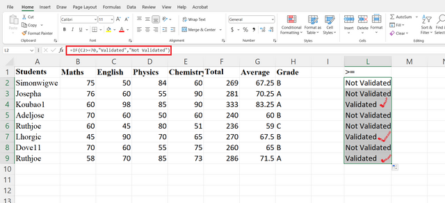
Here the opposite is done for the less than equals to function. But then we are going to employ the formula
=IF(C2>=70, "validated", "not validated")`
By mastering this formulas we can be able to navigate our way through Excel with ease.
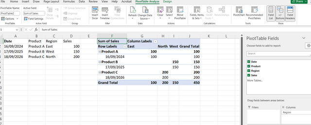
Based on the given data below: Create a pivot table that shows (see) total sales by product, by dragging the product to the Rows areas, Region to the Column area, and Sales to the Values area. Please we want to see the steps taken in adding the pivot table.

To begin with, we start by recreating the table and then applying the various tasks explained.
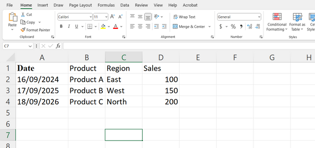
We proceed The insert tab , And then click on pivot tables .
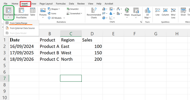
Next, we select the range of our data in the dialogue box, and then it's up to us to put it in the same sheet or on a separate sheet. I will install mine on the same sheet.
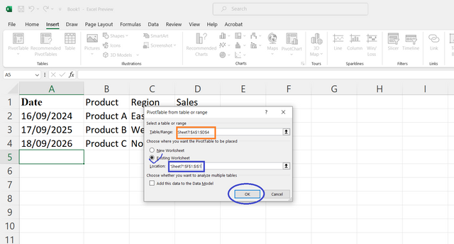
After selecting our data range I then click on ok. Www will be generated automatically. Mama, this is me on Monday?
I then select the region Which are required and then everything is okay.
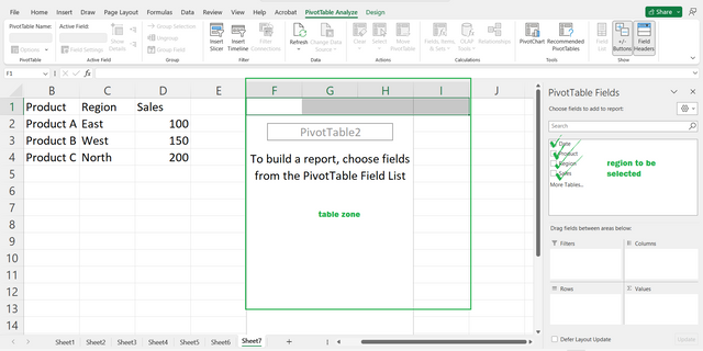
After selecting, our table will appear As seen below.
By navigating These formulas, We can be able to produce and assess more data using the Excel It fields like; organizing data, perform calculations, analyze trends, and create visualizations has made it indispensable in various fields, from finance and accounting to education and research. Whether you're managing a small business, analyzing scientific data, or simply tracking personal expenses, Excel can help you achieve your goals efficiently and effectively.
I would like to invite a following person to join me participate in this contest. @chant, @fombae and @wirngo
Best regards: @rafk
</div
@tipu curate
Holisss...
--
This is a manual curation from the @tipU Curation Project.
Upvoted 👌 (Mana: 5/8) Get profit votes with @tipU :)
Upvoted. Thank You for sending some of your rewards to @null. It will make Steem stronger.
This post has been upvoted/supported by Team 7 via @httr4life. Our team supports content that adds to the community.