SEC | S20W2 | Data Analysis with Google Sheets: (Advanced Excel formulas, and pivot tables)

Hello everyone! I hope you will be good. Today I am here to participate in the contest of @josepha about the Data Analysis with Google Sheets. It is really an interesting and knowledgeable contest. There is a lot to explore. If you want to join then:

---

---

Join Here: Data Analysis with Google Sheets: (Advanced Excel Formulas, and Pivot Tables )

---

---

Designed with ^Canva

Explain what you understand by Advanced Excel Formulas, and show us where advanced formulas such as the lookup function, and logical function are found in Excel with clear screenshots.

Advance formulas of Excel help the the users to perform the complex calculations in seconds. These advance formulas are used for the data analysis and automation in the spreadsheets. These formulas include basic arithmetic operations. And they allow dynamic data manipulation. We can use conditional logic with the help of the advance formulas as well as they are used to retrieve the data from the large datasets which are complex and one cannot find the data easily by manual try. So using the advance formulas we can separate the data from the complex datasets as well as we can perform complex calculation in seconds.

Lookup Functions

Lookup functions are used for searching and retrieving data from specific locations in the table or a provided range. They are useful when we deal with the large datasets where manual searching becomes impossible because of a lot data management and time consuming process. It has different types:

• VLOOKUP

• HLOOKUP

• XLOOKUP

• VLOOKUP: Searches for a value in the first column of a table and returns a value in the same row from a specified column.

  • Syntax: VLOOKUP(lookup_value, table_array, col_index_num, [range_lookup])

• HLOOKUP: It is similar to VLOOKUP. But it searches for a value in the first row of a table and returns a value in the same column from a specified row.

  • Syntax: HLOOKUP(lookup_value, table_array, row_index_num, [range_lookup])

• XLOOKUP: It is an improved version of VLOOKUP and HLOOKUP. It allows searching oif data in any direction by handling exact and approximate matches. It can return multiple results.

  • Syntax: XLOOKUP(lookup_value, lookup_array, return_array, [if_not_found], [match_mode], [search_mode])

Where To Find in Excel

Here is step by step guide to find the LOOKUP Function in the Excel:

• First of all open your Excel Software
• Then move to the Formulas section.
• Select Lookup and Reference with the blue colour.
• All the lookup formulas and other references will appear in a dropdown list.
• All the LOOKUP formulas are avail in that list.

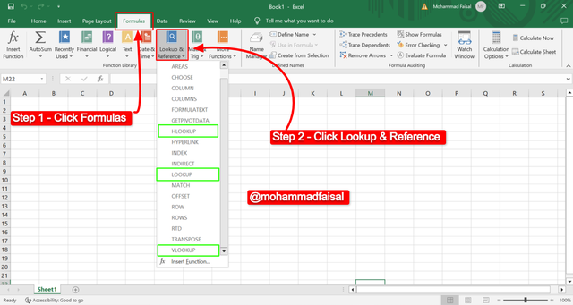
The red arrows are representing the steps and the green boxes are highlighting the LOOKUP Functions in the list. O in this way we can access LOOKUP Functions.

Logical Functions

Logical functions allow the users to perform the action based on the defined conditions. When the certain conditions are met then the required function is executed. They help us in decision making process.

There are different logical functions which are given below:

• IF: It performs a logical test and return one value according to the condition.

  • Syntax: IF(logical_test, value_if_true, value_if_false)

• AND: It returns TRUE if all specified conditions are true and FALSE if all the conditions are FALSE.

  • Syntax: AND(logical1, [logical2], ...)

• OR: It returns TRUE if any of the conditions is TRUE and return FALSE if all the conditions are FALSE.

  • Syntax: OR(logical1, [logical2], ...)

• NOT: It reverses the logical values. If one value is TRUE it changes it to FALSE.

  • Syntax: NOT(logical)

• IFERROR: It returns that specific value which we set when an error occurs.

  • Syntax: IFERROR(value, value_if_error)

It is same finding logical functions as well with a minor difference. Here is step by step guide to find the Logical Function in the Excel:

• Open your Excel Software
• Access the Formulas section at the top of the menu.
• Then find Logical section in the menu of Formulas.
• Click on the purple icon named Logical with the ? mark as its icon.

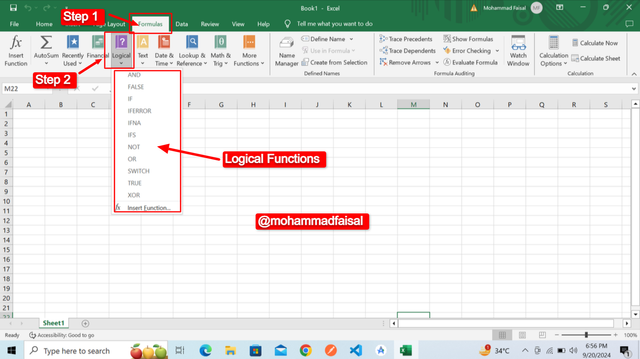
So it is how we can find the logical functions in the excel. And we can use them according to our requirements.

---

Write the IF Function formula to calculate the total, average score, and grade of students given in the table below.

Students	Maths	English	Physics	Chemistry
Simonnwigwe	75	50	84	60
Josepha	76	60	55	90
Kouba01	60	98	85	90
Adeljose	70	60	50	60
Ruthjoe	60	45	80	51
Lhorgic	45	90	70	65
Dove11	70	60	55	75
Ruthjoe	58	70	85	73

As we know that IF is a logical function and we cannot use it with the arithmetic calculations. We can only use it to find the conditions whether one condition is true or false. So I willuse it to find the grades by writing some conditions for the grades. And to find the total and average score I will use sum and average formula. SO lets start calculating it.

Total Calculation

In order to find the total score of the students we can sum up all the scores of the subjesct which are Math, English, Physics and Chemistry. So in order to sum up these scores we use the formula =SUM(B2:E2) in excell.

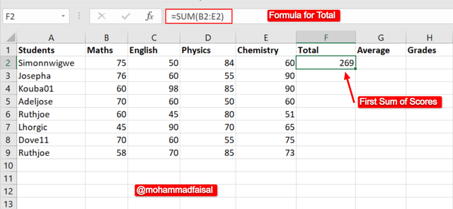
I have inserted all the given data in the tabular form in the excell. Then in order to calculate the total of the scores I have applied the =SUM(B2:E2) formula for the first participant and it has successfully calculated the sum.

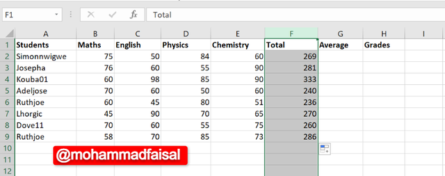
To find sum of scores of all the students I have simply dragged down the top box up to last. And it has calculated the sum of all the students.

Average Calculation

AS we know that we calculate average in mathematics by summing up all the given values and then dividing them on the number of the quantities. So in excel it is also same but we can manage it with a single formula. The formula to calculate the average is =AVERAGE(B2:E2). So let's calculate the average.

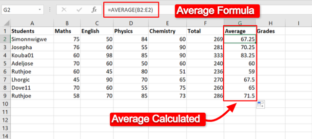
Here again I put the formula in the average section and it automatically calculated the average of the scores. Then i dragged down it up to last and it continued to calculate the average of all the students. And final output is there in the screenshot.

Grade Calculation Using IF Function

We can calculate the grades of the students using IF function. Here I have selected some criteria to calculate the grades of the students:

A if the average score is 80 or above.
B if the average score is between 70 and 79.
C if the average score is between 60 and 69.
D if the average score is between 50 and 59.
F if the average score is below 50.

For this criteria the formula is given below:

=IF(G2>=80, "A", IF(G2>=70, "B", IF(G2>=60, "C", IF(G2>=50, "D", "F"))))

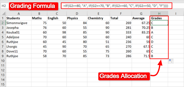
So it is how we can calculate the grades of the students. We can define the conditions for the grades allocation and then we can execute the code accordingly.

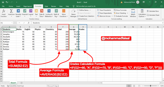
Here all the required functions has been executed to calculate the Total, Average as well as the Grades of the students according to their marks average.

Briefly discuss four IF function Operators that you have learned and tell us their functions and when we are to use them

Here are 4 important operators which we can use with IF function:

• Greater Than (>)
• Less Than (<)
• Greater Than or Equal TO (>=)
• Equal (=)

Greater Than (>)

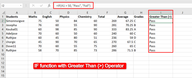
Greater than operator is used to check if one value is greater than other value. For example IF(A1 > 50, "Pass", "Fail"). This condition checks if the value of A is greater than 50 then it shoud retur pass otherwise fail.

Less Than (<)

Less than operator is used to check if one value is less than the otehr. For example: IF(A1 < 50, "Low", "High") This condition checks if the value A1 is less than50`.

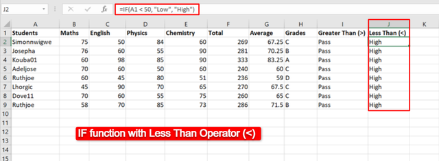
Greater Than or Equal To (>=)

This operator is used too check the value if one value is greater than or equal to other value. For example IF(A1 >= 70, "Distinction", "Regular") This condition checks if the value of A1 is greater than or equal to 70 and return the output accordingly. We can use it for the grading purpose.

Here you can see the greater than equal to operator worked with the If function and it has given different values according to the predefined condition. Similarly have changed the values in the previous sections as well.

Equal To (=)

This operator is used to check the if two values are equal to each other or not. For example: IF(A1 = "Yes", "Approved", "Pending") This checks if the value in A1 is equal to Yes. So we use this operator for checking the exact values.

Here I have used equal operator to check if the student is pass then the student has been approved otherwise the student is in the pending list.

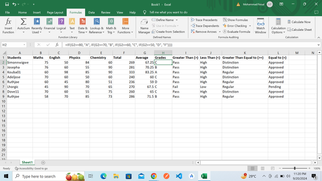
It is the complete excel sheet which is representing the student table with the total, average marks as well as grades of the students. It is also representing the usage of the 4 different operators with the IF Function.

---

Based on the given data below: Create a pivot table that shows (see) total sales by product, by dragging the product to the Rows areas, Region to the Column area, and Sales to the Values area. Please we want to see the steps you take in adding your pivot table.

Date	Product	Region	Sales
16/09/2024	Product A	East	100
17/09/2024	Product B	West	150
18/09/2024	Product C	North	200

It is very easy to create a pivot table for the given data. As we already have a data so let's start making the pivot table that will show the total sales by product, region and sales. So we can follow these steps:

Step 1: The first step to create a pivot table is to have the data in a correct tabular form in Excel.

So here you can see that first of all I have added all the data in the tabular form in Excel.

Step 2: After writing the data in the tabular form we need to insert pivot table.

• To insert pivot table we need to open the Insert section as it can seen in the below image.

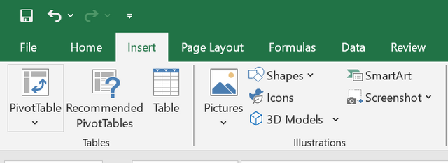
• It is showing 3 options but we have to choose pivot table.

Step 3: We need to give the range to the pivot table. You can see in thebelow image the pivot table is demanding the range of the table.

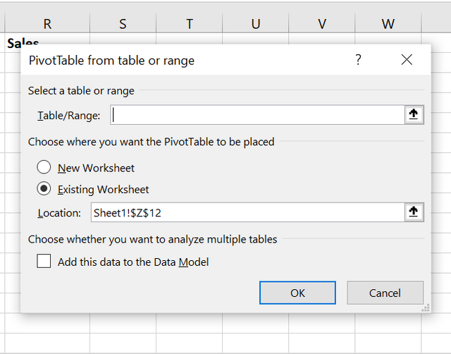
To add range of the table we follow these further steps:

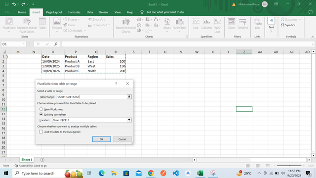
• Select the table which you have created for your data. It will automatically get table or range from that selected table.

• You can see in the pivot table pop up that the range of the table has been added to the pivot table which is Sheet1!$O$1:$R$4 and this range can vary depending upon the size of data or the number of rows and columns of the table.

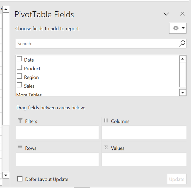
Finally the pivot table has been added and now we have to select our required attributes to show in the table. And here we can see the fields of the pivot table.

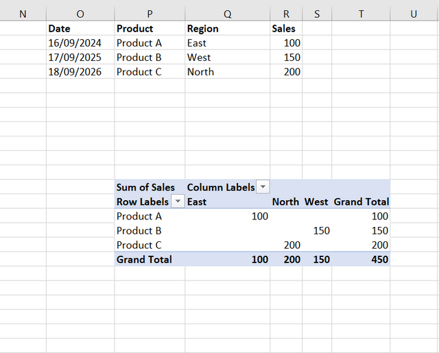
I have added the pivot table fields into the it. I have dragged the product to the rows field. Similarly I have added Region to the columns area. And the sales to the values to find the sum of the values of each region.

• The rows show different products such as Product A, Product B, and Product C.

• The columns show the different regions such as **East, North and West.

• The value areas contains the sum of the sales for each product per region.

Furthermore we can change the format of the pivot table and this process gives us dynamic summary of the sales data broke down by product and region.

---

Conclusion

There are different types of functions which are used in the spreadsheet. Logical and LOOKUP functions are one of them. These both are of great importance. LOOKUP functions are used for the searching purposes and similarly logical functions are used for the decision making and too check the conditions. There are different operators which we use with other logical functions such as IF to solve the complex queries. These functions speeds up our work and save us from time wasting because of their automated working. Pivot tables are also great sources to sort the data according to our needs.

---

Disclaimer: All the screenshots have been taken from Desktop Excel software otherwise stated.

---

I invite @kouba01, @sergeyk and @stream4u to join this contest of spreadsheets.

Best Regards: @mohammadfaisal