Data Analysis with Google Sheets: (Advanced Excel Formulas, and Pivot Tables )
Topics Covered: Advanced formulas, and pivot tables.

This comes to the second week of our lessons and we humbly welcome you here once again. In our previous lesson, we only introduced you to the basic formulas of spreadsheets this time around we will be looking at more advanced formulas, pivot charts, and data analysis.
Having said that, Advanced Excel formulas are rarely used because of how uncommon they are been used. There are inbuilt formulas that you can use to retrieve specific data from an existing data set which is like duplicating the data, filtering the data, and so on. You can also use these functions which we will practically look at to create a dashboard, generate reports, and so on.
 |  |
|---|
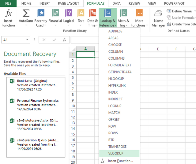
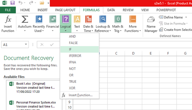
For example, looking at the above images you can see some of the inbuilt advanced Excel formulas that you can use. Also, these inbuilt formulas are available in LibreOffice and not just in Excel. Out of the many advanced Excel formulas we have let's practically talk about these two VLOOKUP formula and the IF FUNCTION formulas in this lesson.
VLOOKUP Formula in Excel
Based on simplicity VLOOKUP is the most used formula in Excel. Simply this is the formula that helps you to search for the in the leftmost column of the table array and returns the value from the same row from the specific columns.
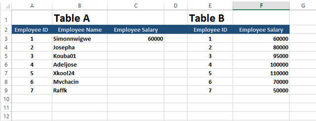
Let's consider looking at the short example in which we have applied this formula. Now for example, we have two different tables that contain the names, employees ID, and salary of employees, as our main column and we want the salary from our table B to be in table A.
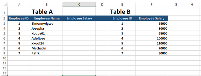
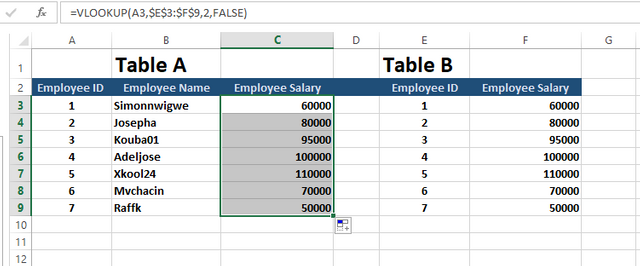
By mainly looking at the data above, if we want to get the salary in Table B in Table A, we will have to apply the formula shown in the image below.
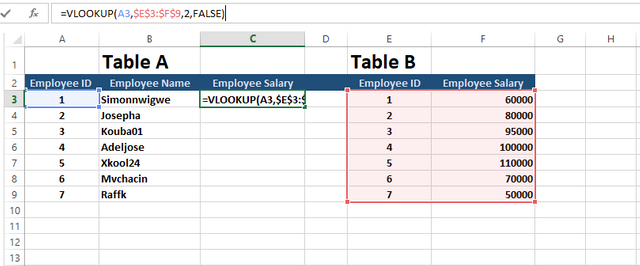
Now, once you have entered the formula in employee salary which is cell C, you can drag the formula to the rest of the cells to get your results in each cell which is the salary of employees.
Using the IF Function
One of the most powerful features of spreadsheets is the ability to perform different calculations based on changing values. IF Function is what is mainly used. This function makes logical tests of evaluation and performs one of two different calculations based on the result. The format for the IF Function is stated 👇 below.
=IF(logical text,value if true, value if false)
The logical text is what specifies what the statement of the IF Function will evaluate for you.
The Value If True, If the logical Text is found to be true, then the result of your IF Function will be whatever is in the format we have shared.
The Value If False, If the logical test is found to be false, then the result of your IF Function will be whatever is in the format we have shared.
Comparison is what the logical test mostly uses which helps us to obtain our desired result. What is used to identify or define different types of data is Qualifiers which are punctuation marks. For instance, text that is used in a formula needs double quotes as qualifiers. Having said so let's take a look at the comparison operators that you can see in IF Function.
- Equal to (=)
- Greater than (>)
- Less than (<)
- The greater than or equal to (>=)
- Not equal to (<>)
- The less than or equal to (<=)
Now let's learn how to create a simple assessment report using a spreadsheet which will then apply the IF Function.
- First is for us to identify student information in the report.
- Secondly is to open MS Excel
- Thirdly enter the data shown below.
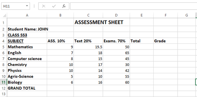
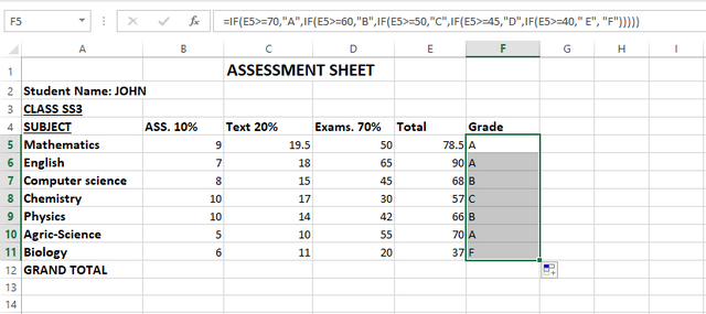
From the above data, to find the total. Select cell E5 and enter the formula =Sum(B5:D5) and press enter. The total score should appear in cell E5. Using the formula Excel will add the contents in B5, C5, and D5 and provide you with the answer.
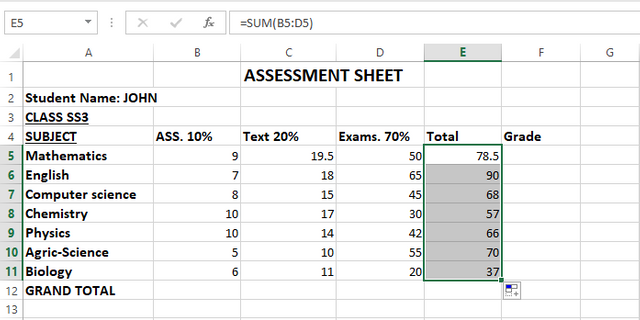
Converting the percentage to a level score of 1, 2, 3, or 4 which can also be alphabetic grade A, B, C, and so on. Now to do this, we will have to first determine our range.
- 70% -100% = A
- 60% - 69% = B
- 50% - 59% = C
- 45% - 49% = D
- 40% - 44% = E
Anything else less than that which is given above should be F.
To get this, we will have to click on cell F5 and type in the given formula below using the If function.
=IF(E5>=70, "A", IF(E5>=60, "B", IF(E5>=50, "C", IF(E5>=45, "D", IF(E5>=40, "E", "F")))))
Once you have entered the formula correctly you need to click on the Enter key and you will get the right results which you can then drag down to get other results as shown below.
Pivot Table
Now we have moved to the pivot table which is a summary tool that helps us to synthesize information from a database or set. Summary means all kinds of descriptive statistics data that help pivot table groups together in a meaningful way. If you are a data analyst you can use a pivot table to summarise large datasets into a meaningful table that can be easy to view.
Pivot tables are used for some of the following reasons given below.
To group data into categories.
To count the number of items in each category.
To sum the value of items.
To find minimal or maximal value, compute average, etc.
To create a pivot table in a spreadsheet (excel or LibreOffice), you will need to follow the steps shared below.
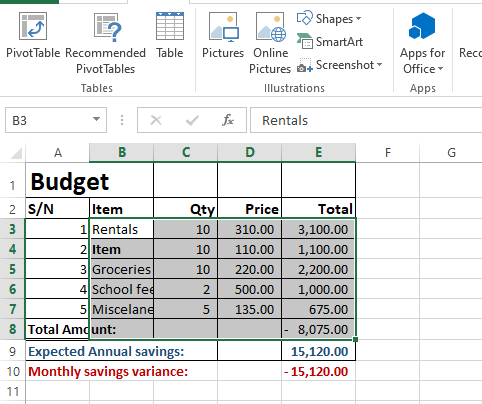
Prepare your data
You have to make your data well organized in a tabular form, with column headers for example; Date, Product, Sales, and so on.
Each of the column headers should represent a specific variable, whereas each row should represent a unique record.
Select Your Data
- At this stage you will have to highlight the day range that you want to analyze.
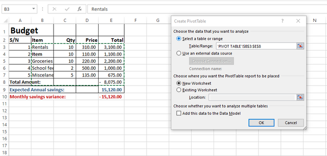
Insert The Pivot Table:
The below steps are what you need when inserting a pivot table in Excel.
On the ribbon you click on
InsertClick on
Pivot TableConfirm the range of your data in the dialog box, and choose to either place the pivot table in an already existing worksheet or a new worksheet.
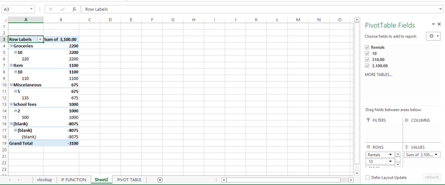
Choose Pivot Table Fields
Once you have created your pivot table, you will see a new pane that will appear allowing you to drag the field into 4 areas.
Row: The data categories that you want as row labels.
Column: The data categories that you want as column.
Values: The data you want to aggregate.
Filters: This allows you to view specific data only.
Customise your pivot table
You can do this, by changing the calculation type
Applying filters and formatting.
Now let's take a look at the below example.
 |  |  |
|---|
From the above screenshots, you can see how we have applied a pivot table in the given example.
Explain what you understand by Advanced Excel Formulas, and show us where advanced formulas such as the lookup function, and logical function are found in Excel with clear screenshots.
Write the IF Function formula to calculate the total, average score, and grade of students given in the table below.
| Students | Maths | English | Physics | Chemistry |
|---|---|---|---|---|
| Simonnwigwe | 75 | 50 | 84 | 60 |
| Josepha | 76 | 60 | 55 | 90 |
| Kouba01 | 60 | 98 | 85 | 90 |
| Adeljose | 70 | 60 | 50 | 60 |
| Ruthjoe | 60 | 45 | 80 | 51 |
| Lhorgic | 45 | 90 | 70 | 65 |
| Dove11 | 70 | 60 | 55 | 75 |
| Ruthjoe | 58 | 70 | 85 | 73 |
Briefly discuss four IF function Operators that you have learned and tell us their functions and when we are to use them.
Based on the given data below: Create a pivot table that shows (see) total sales by product, by dragging the
productto the Rows areas,Regionto the Column area, and Sales to the Values area. Please we want to see the steps you take in adding your pivot table.
| Date | Product | Region | Sales |
|---|---|---|---|
| 16/09/2024 | Product A | East | 100 |
| 17/09/2024 | Product B | West | 150 |
| 18/09/2024 | Product C | North | 200 |
Posts must be published in your blog and not in any community.
The title must be: "SEC | S20W2 | Data Analysis with Google Sheets: (Advanced Excel formulas, and pivot tables.)
The post must contain a minimum of 350 words, be free from plagiarism, and not use Artificial Intelligence (AI) or other forms of cheating.
Use the main hashtag #spreadsheet-s20w2 (required) among the first 4 tags
Add your country name hashtag (e.g. #nigeria)
If using the hashtag #burnsteem25 make sure you give 25% of the reward to @null
Invite 3 friends to participate.
Paste your participation link in the comment section, and don't forget to Vote and Rate this post.
This contest starts Monday, September 16, 2024, at 00:00 UTC and ends on Sunday, September 22nd, 2024, at 23:59 UTC."
Note: We will choose the winners based on the quality of the post, a quality post in our opinion is a post that can provide interesting ideas and new insights for its readers. Proper use of markdown is also part of the quality of a post.
Cc:-
@simonnwigwe
https://steemit.com/spreadsheet-s20w2/@nahela/sec-or-s20w2-or-data-analysis-with-google-sheets-formulas-avanzadas-de-excel-y-tablas-pivotantes
Segunda semana :)
Check closing date...
Thank you. Corrected as suggested.
My entry
https://steemit.com/spreadsheet-s20w2/@rafk/sec-or-s20w2-or-data-analysis-with-google-sheets-advanced-excel-formulas-and-pivot-tables
Excelente temática para esta segunda semana del curso; conocer el funcionamientos de las fórmulas avanzada, la función SI y las tablas dinámicas, son elementos que nos serán de gran utilidad para trabajar con grandes cantidades de datos en las hojas de cálculo.
Desde ya comienzo a preparar mi participación. Saludos.
Wonderful topic for week2. For those of us that struggling to be a computer literate this is a golden opportunity for us. I will surely do my best in this week's own.
tema yang menarik dan seperinya lebih sulit dari minggu sebelumnya.
Saludos!!!
Excelente clase, y seguimos avanzando en funciones, herramientas muy útiles de excel, me ha encantado, ya que he aprendido herramientas que no conocía.
Bendiciones.
Hello, below you can find my entry:
https://steemit.com/spreadsheet-s20w2/@ady-was-here/sec-or-s20w2-or-data-analysis-with-google-sheets-advanced-excel-formulas-and-pivot-tables
Thank you
Saludos.
El ejemplo de la tabla pivote no se observa claramente, no logro detallar las imágenes, están muy pequeñas.
Another new and interesting task. We are excited to take part. Thanks for this deep explanation of the advanced formula and on pivot table. Entry loading.