SEC | S20W2 | Data Analysis with Google Sheets: (Advanced Excel formulas, and pivot tables.)

It's the second week of SEC and in this post I will show you the assignments of Data Analysis with Google Sheets: (Advanced Excel Formulas, and Pivot Tables ) by @josepha.
Homework
First point
Explain what you understand by Advanced Excel Formulas, and show us where advanced formulas such as the lookup function, and logical function are found in Excel with clear screenshots.
From my perspective the Advanced Excel Formulas are a set of tools/mechanisms used for complex data handling, the best area that I can think of where these are used to their fullest and help a lot is in the financial area, and areas that work with big data structures. These formulas are far more complex than the Basic Excel Formulas we used in the previous week (SUM, AVERAGE etc)
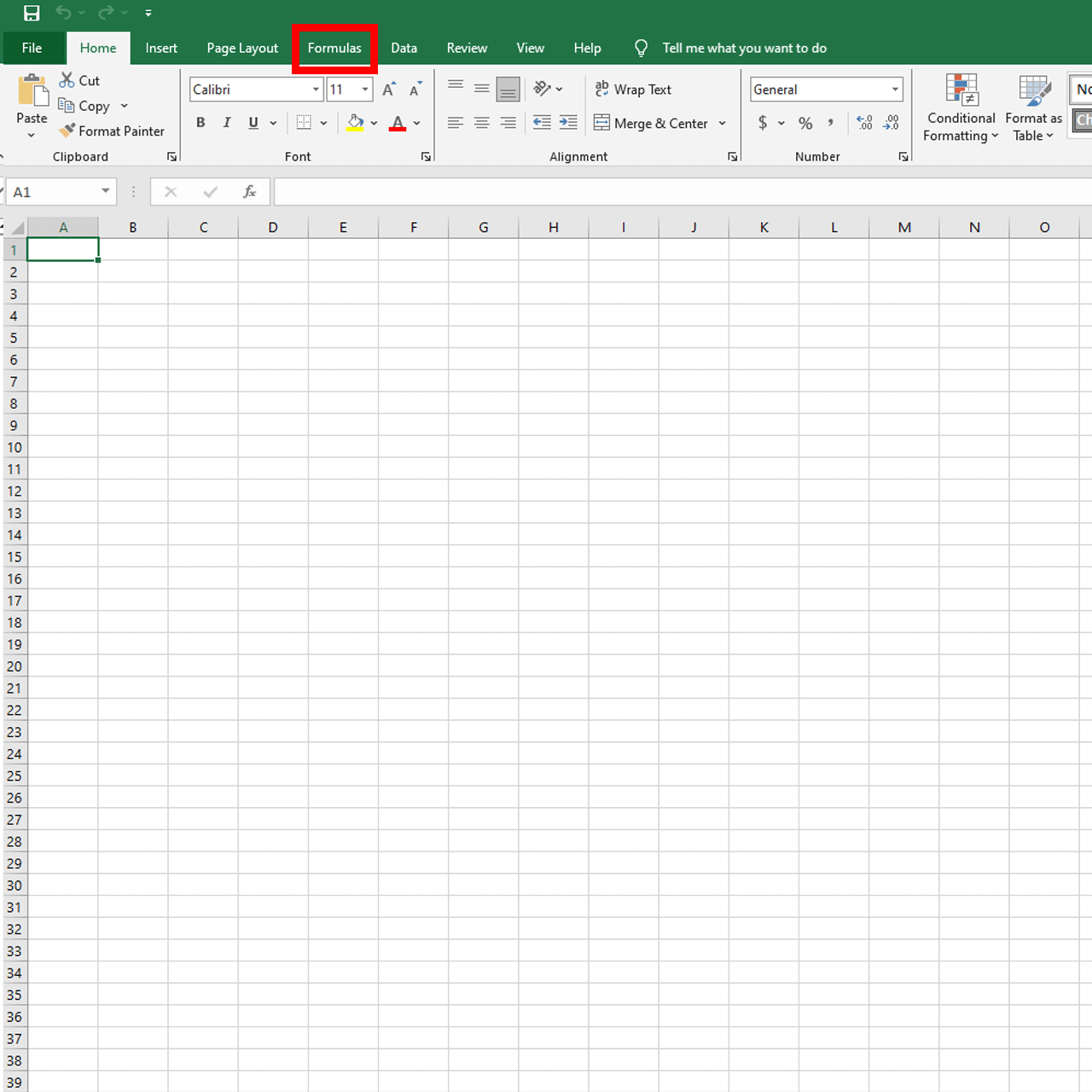
In my version of Excel it is pretty easy to get to the Lookup function. At the top of your Excel window you have a menu with multiple tabs, in this menu we are looking for the FORMULAS tab.
On the FORMULAS tab we are looking for a magnifying glass icon with the "Lookup & Reference" text under, clicking it will open a drop down menu with multiple functions, in these list of functions you'll see the Lookup one.
See the attached GIF above for further explanation!

Now for the Logical function we are going to use the same path as for the Lookup one.
At the top of your Excel window you have a menu with multiple tabs, in this menu we are looking for the FORMULAS tab.
On the FORMULAS tab we are looking for a question mark icon with the "Logical" text under, clicking it will open a drop down menu with multiple functions.
See the attached GIF above for further explanation!
Second point
Write the IF Function formula to calculate the total, average score, and grade of students given in the table below.
| Students | Maths | English | Physics | Chemistry |
|---|---|---|---|---|
| Simonnwigwe | 75 | 50 | 84 | 60 |
| Josepha | 76 | 60 | 55 | 90 |
| Kouba01 | 60 | 98 | 85 | 90 |
| Adeljose | 70 | 60 | 50 | 60 |
| Ruthjoe | 60 | 45 | 80 | 51 |
| Lhorgic | 45 | 90 | 70 | 65 |
| Dove11 | 70 | 60 | 55 | 75 |
| Ruthjoe | 58 | 70 | 85 | 73 |
- We can easily copy the table inside our excel sheet, it will look pretty ugly at first but with a few tweaks we can make it clear.
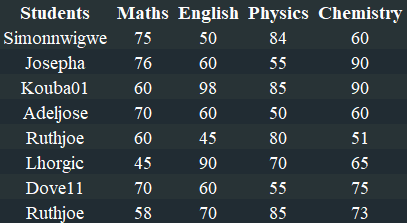

- Now that we have created the table inside our sheet, let's add the AVERAGE and GRADE columns.
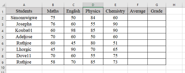
- Time to add the MAGIC, for the Average score we are going to use the AVERAGE formula. In this case we apply the AVERAGE formula on the F2 cell and take the cells from B2 to E2 to cover all the subjects, the formula looks like this:
=AVERAGE(B2:E2)
- We have the first AVERAGE, it's time to drag it to all the remaining cells, this way we get the AVERAGE for each student.
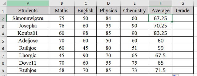
- Let's grade the students, we are going to apply the IF presented in the course, in my case I will apply it on the second row (first student) like this:
=IF(F2>=70, "A", IF(F2>=60, "B", IF(F2>=50, "C", IF(F2>=45, "D", IF(F2>=40, "E", "F")))))
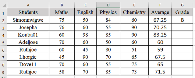
We get the result for the first student, which is B, and it's correct since we apply the B if the AVERAGE is greater or equal to 60, 67.25 is greater than 60 but lower then 70, if it were to be greater or equal to 70, the grade would have been A.
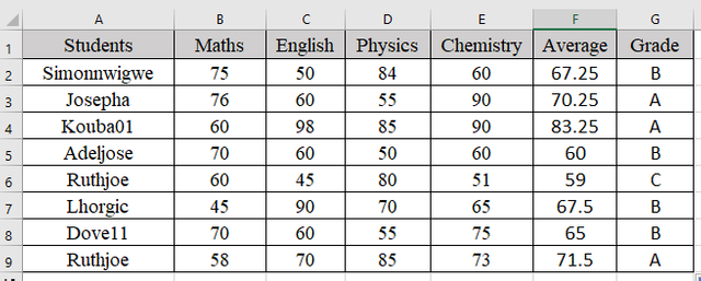
After this we apply it to the whole class and we get this result:
Third point
Briefly discuss four IF function Operators that you have learned and tell us their functions and when we are to use them.
The operators that we can use in an IF statement are the following:
= <> > <
- Equal ( = )
- the equal operator is used to check if two values are equal (exactly the same value)
- example:
=IF(B2 = 100, "True", "False")this statement returns "True" if B2 equals to 100, "False" otherwise
- Not Equal ( <> )
- the not equal operator is the opposite of equal, we check if two values are not equal (not exactly the same value)
- example:
=IF(B2 <> 100, "True", "False")this statement returns "True" if B2 is not 100, "False" otherwise
- Greater than ( > )
- the greater than operator is used to check if one value is greater than another
- example:
=IF(B2 > 100, "Higher value", "Lower value")this statement returns "Higher value" if B2 is greater than 100, "Lower value" otherwise - can be used in combination with the equal symbol ( = ) to check if a value is greater or equal than
- Less than ( < )
- the less than operator is used to check if one value is less than another
- example:
=IF(B2 < 100, "Low", "High")this statement returns "Low" if B2 is greater than 100, "High" otherwise
Fourth point
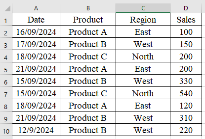
Based on the given data below: Create a pivot table that shows (see) total sales by product, by dragging the product to the Rows areas, Region to the Column area, and Sales to the Values area. Please we want to see the steps you take in adding your pivot table.
| Date | Product | Region | Sales |
|---|---|---|---|
| 16/09/2024 | Product A | East | 100 |
| 17/09/2024 | Product B | West | 150 |
| 18/09/2024 | Product C | North | 200 |
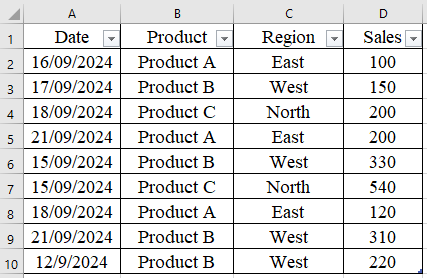
I added the table from the Homework section and added a couple more entries inside it to make it bigger. We now have 9 entries in the table, and before we can Pivot it we need to create the table headers.
To do the Table Headers we can either use the Table option present in the Insert tab, or use the CTRL+T shortcut.
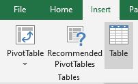
We created some headers in our table but Excel doesn't know that these are headers until we define them. In order to do that we have to select the whole table (all the data that we added), with everything selected we use the Table option or the shortcut mentioned above.
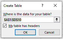
A new window will pop up with the range of your table, make sure the option "My table has headers".
Your table should change a little, it should look like this, you can see the new arrows my table has at the headers.
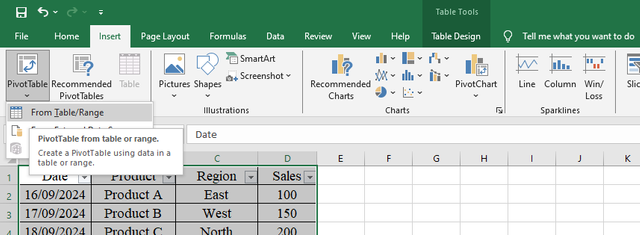
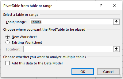
Now, again select the whole table and from the insert tab we can use the Pivot option -> From table/range:
A new window will pop up, you don't really need to make any changes here, only if you have something specific that you need.
The interface of your Excel will change a little, now we can move everything accordingly:
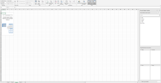
The new interface
Now the assignment tells us to do the following:
- drag the Product to the Rows area
- drag the Region to the Column area
- drag Sales to the Values area
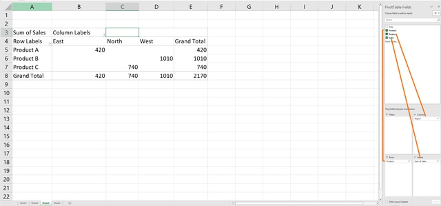
The final result, I know it's not colored like in other people's examples but in my case these are the settings of my Excel
In the end I would like to invite @titans @mojo-ciocio and @r0ssi.
Thank you @josepha and @simonnwigwe for this week's course!
I'd also like to thank everyone who stopped by, wishing you all the best!
Upvoted! Thank you for supporting witness @jswit.
Congratulations! Your post has been upvoted through steemcurator06.

Good post here should be . . .
Curated by : @𝗁𝖾𝗋𝗂𝖺𝖽𝗂
Thank you @heriadi and Team-4!