SEC | S20W1 | Spreadsheet Essential For Beginners (Spreadsheet Overview, Spreadsheet Interface & Basic Formulas)
This is my homework post for Professor @simonnwigwe’s Season 20 Week 1 teaching class assignment, Spreadsheet Essential For Beginners.
Note :
- I performed this task on Windows 10 PC, Microsoft Excel 2021, and Google Chrome.
Task 1 - Explain your understanding of the Spreadsheet, listing its features, its purposes, and an example image that follows your explanation.
Spreadsheet is a very useful application especially for office work needs. There seems to be no office that does not use this type of application because it will help them in many ways, including making financial reports and progress achieved.
Its capabilities include managing complex data (numeric or text) in tables stored in cells. The functions it has make work very easy, saving a lot of time. The most popular spreadsheet application is probably Excel released by Microsoft Corporation. Besides that, we can also mention Google Sheets which as the name implies is a product of Google, LLC. Another one that is no less popular and open-source based is LibreOffice Calc.
Sources: MS Excel | Google Sheets | LibreOffice Calc
There are tons of features in Spreadsheet that help it handle complex tasks, including:
- Columns, Rows, Cells. The simplest feature is probably the visual feature of rows, columns and cells. Rows and columns make a Spreadsheet interface look like a table. Rows are horizontally aligned and named with numbers while columns are vertically aligned and named with letters, and the cross between rows and columns is called a cell and named with a combination of letters and numbers.
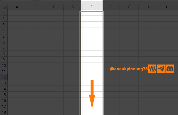
Column E
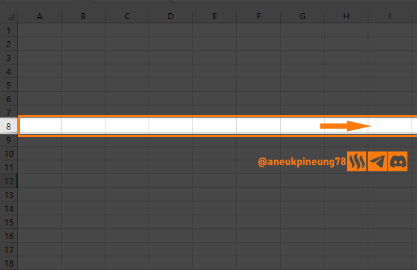
Row 8
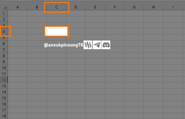
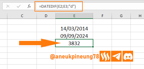
Cell C4 - Formulas. Spreadsheet is equipped with lots of formulas that can be used for various needs, from simple ones such as the one used to find the number of cells that have contents in a certain cell range, to complex ones such as to find how many product A sold in outlet 10 in the last month based on the data in a table, for example. The following image gives an example of another simple formula, which is the formula to calculate the distance between two dates in term of days.
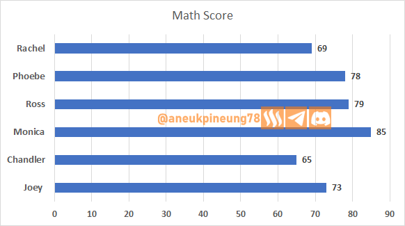
- Diagrams and Graphs. Work reports would be very boring if they only contained numbers and letters. To bring more value to these reports, Spreadsheets have the ability to convert data into diagrams and graphs. Here is an image that shows a simple graph of 6 students' math scores.

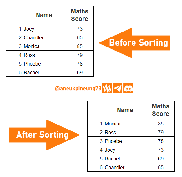
Simple Chart - Sorting. There are times when data needs to be sorted from the lowest value to the highest value or vice versa, either numerically or alphabetically. With Spreadsheet this can be done easily. The following image shows the state of 6 students' math score data before and after sorting from highest to lowest. Sorting like this is useful in ranking, for example related to work performance, progress, and so on.


And there are many more Spreadsheet features that help work.

Task 2 - Based on the basic Formulas given in this lecture, use the data below to calculate the SUM Function and the AVERAGE Function of the class. Show clear working as to how you arrive at your answers.
| A | B | C | |
|---|---|---|---|
| 1 | Name | Maths Score | |
| 2 | ruthjoe | 60 | |
| 3 | bossj23 | 65 | |
| 4 | sahmie | 59 | |
| 5 | okere-blessing | 79 |
Sum and Average are two of the important and popular functions in spreadsheet applications.
SUM
The SUM function, which is useful for finding the sum of numbers contained in the cells in question, can be done in three ways:
- activate the sum formula [
sum=(] followed by the selection of cells that contain the data that needs to be summed. This is used in a condition where the cells that have the data you want to sum are in random positions or have gaps (separated by cells that have unwanted data). - activate the sum formula [
sum=(] followed by selecting the cell range. This method is used when the cells that have data are in a range that is not separated by cells that have unwanted data. - combination of the two methods above, if the case has such complexity.
In the case example given by Professor Simonnwigwe, of course it makes more sense if I use the second method, which is utilizing the cell range in the formula, this method is simpler. Although the first method as I mentioned above can also be used, but this method is more time-saving and “smarter”. What you need to do is just a few easy steps:
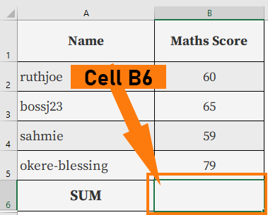
- First, determine the cell where the SUM result will be placed, here I use cell B6.
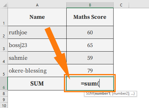
- Second, activate the SUM function by typing
=sum(.
- Third, select the first cell and while pressing the [Shift] key on the keyboard (Windows) press the arrow on the keybord in the direction where the next cells are (in my case, upwards), after all the desired cells are selected, end the function with a closing parenthesis
)and press the [Enter] button. Such a method is suitable in cases when the cells have a short range (maybe up to 10 cells, but this is subjective). For data located in cells that have a long range, for example 20 cells (for me this is already a long range), then I think it is more effective to select the first cell and then by still pressing [Shift] select the last cell where the desired data is located, then press the [Enter] button.
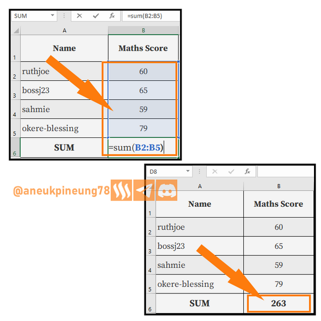


This operation produces the value 263. Here is a video that shows how I do this.
Average
The Average function as the name implies is to find the average value of a set of data. The calculation method is similar to the use of the SUM function, which is to invite the necessary cells into the AVERAGE formula, either by adding cell by cell or by adding a cell-range or a combination of both, depending on the need.
The following video shows how I use the AVERAGE function for the data provided in the task, different from the method I use in using the SUM function, this time I will click the first cell and the last cell (not using the arrow keys). So the steps are:
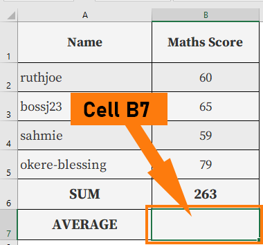
- First, determine the cell where the AVERAGE value of the data will be placed, here I use cell B7.
- Second, activate the AVERAGE function by typing
=average(.
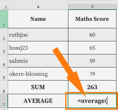
- Third, select the first cell and while pressing the [Shift] key press the last cell of the cell range. Release the [Shift] button, end the formula with a closing bracket
), and press [Enter].


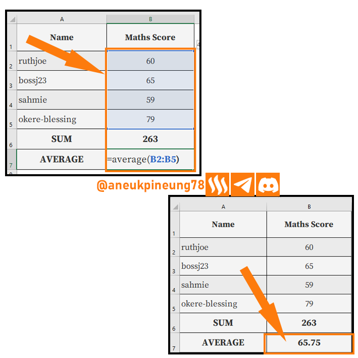
We get the AVERAGE value of 65.75.
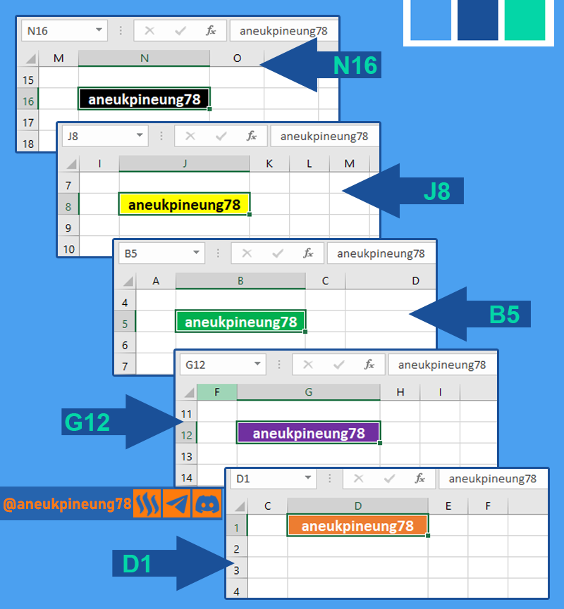
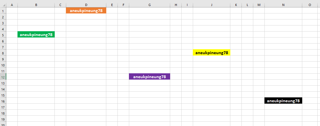
Task 3 - Take a screenshot of your worksheet and identify the cell Addresses of the following; N16 with a fill color of black, J8 with a fill color of yellow B5 with a fill color of Green G12 with a fill color of purple and D1 with a fill color of orange. Write your username on these cells using a visible font.
The individual screenshot of the target cells are shown in the image below.
The screenshot below shows the worksheet that contains all the target cells.
This task reminds me of a rather funny story that happened a long time ago. One day, my boss asked me why she couldn't see anything in the cells in the worksheet while the formula bar showed the data. Then I directed her to change the text color or the cell's background color, she laughed loudly, I think she was joking with me.
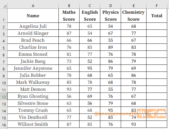
Task 4 - Prepare a score for 15 students where the cell A1 label will be Name, cell B1 label will be Maths Score, cell C1 label will be English Score, cell D1 label will be Physics Score, cell E1 label will be Chemistry Score and cell F1 will be labeled Total. Add all necessary information and calculate the total for each student. Show clear working.
I have a table of students' names and their grades for each subject as shown below.
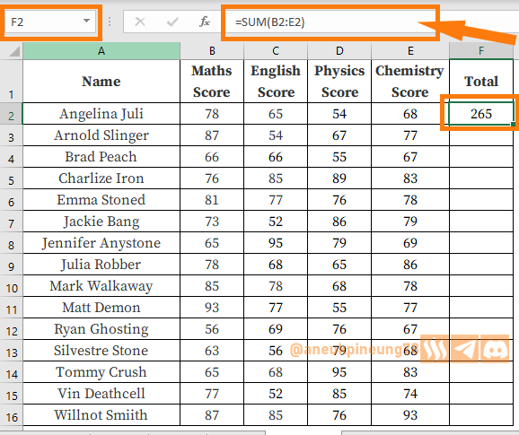
Next, to fill in the total value obtained by each student, I will use the SUM function. The steps I take are:
- First, I run the SUM function for the students in the topmost order (Angelina Juli) whose results are displayed in cell F2, by using the cell range in the SUM formula, I get this formula:
=sum(B2:E2).
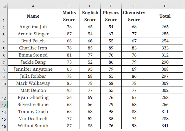
- Second, I duplicate the formula to be used in finding the total score for the rest of the students. This can be done by copying cell F2 and then pasting it to cell range F3:F16, or it can also be done by dragging the formula in cell F2 down until cell F16.

The final state of the table is shown in the figure below.
The following video shows how I completed Task 4.
Thanks
Thanks Professor @simonnwigwe for the lesson. I also want to invite @rayfa, @dhisky, and @seribubulan to join.
Pictures Sources
- The editorial picture was created by me.
- Unless otherwise stated, all another pictures were screenshoots and were edited with Adobe Photoshop 2021.


https://x.com/aneukpineung78/status/1834771635259556284
Kalau saya lihat video tutorial excel, saya jadi ingat @paulag. Apa dia masih ngajar excel di internet?
Ngga tahu pastinya tapi beberapa bulan lalu dia masih promosikan kursus online di hive.
Congratulations! Your post has been upvoted through steemcurator06.

Good post here should be . . .
Curated by : @𝗁𝖾𝗋𝗂𝖺𝖽𝗂
Wawww sangat jelas pemaparannya, saya sangat menyukainya. Benar-benar hebat.
Ah biasa saja. Ini hanya laporan yang bisa dibuat oleh siapapun karena Excel adalah aplikasi kantor yang lazim mudah ditemukan saat ini dan ada dalam semua kantor.
Kalau membuat memprakteknya memang sangat mudah pak, tapi menyusun menjadi sebuah kalimat harus screenshoot itu yang bikin malas dan susah.
Orang memang sudah mahir dalam memainkan ms. excel ini,
Merangkai seperti anda ini, sedikit yang mau.
Saya pribadi memiliki sejarah yang tidak pendek dalam blogging, sejak masa-masa awal Blogspot dan Wordpress, saya telah mengelola beberapa blog di masa lalu termasuk beberapa blog organisasi dan beberapa blog pribadi. Blog pribadi saya terdiri dari berbagai kategori bahasan: musik, filem, sastra, tutorial, buku. Tetapi semua telah saya tutup.
Maksudnya adalah saya menyukai menulis. Jadi membuat tutorial seperti ini yang mengharuskan melakukan penangkapan layar dan penciptaan gambar dengan aplikasi, bukanlah sesuatu yang baru dan membuat saya susah, saya justru menikmatinya, walaupun jam tidur saya harus terganggu karenanya.
Merangkai seperti anda ini, sedikit yang mau.
Mungkin bukan hanya perkara MAU atau TIDAK MAU saja, mungkin juga ada variabel lain yang menentukan. Tetapi saya lihat tidak sedikit juga yang telah menciptakan artikel tugas ini dengan kualitas yang lebih baik dari yang saya hasilkan. Saya pikir Professor @simonnwigwe dan Professor @josepha akan menghadapi sedikit kesulitan dalam memilih artikel-artikel terbaik karena banyaknya artikel-artikel berkualitas yang masuk, tapi saya percaya mereka pasti punya metode yang keren dalam menentukan. Ini merupakan awal musim yang hebat, untuk bisa terlibat dalam tantangan ini.
Thanks.
Has realizado muy buena explicación del funcionamiento de las hojas de cálculo y su gran utilidad para diversas tareas, especialmente en la obtención de resultados precisos.
Este tipo de herramientas son claves en la presentación de datos de forma sintetizada por medio de tablas o a través de gráficos.
Éxitos en su participación.
Thanks, dear friend. You yourself wrote an excellent article about this. I wish you the best in life.