SEC | S20W1 | Spreadsheet Essential For Beginners (Spreadsheet Overview, Spreadsheet Interface & Basic Formulas)
Hello everyone, this is my first time ever participating in a SEC. Below I have attached all the steps I made during the Spreadsheet Essential For Beginners homework.

The homework
First assignment
Explain your understanding of the Spreadsheet, listing its features, its purposes, and an example image that follows your explanation.
Well, a Spreadsheet is a grid formed with rows and columns that in the end form cells that can hold data (numbers, characters, formulas etc.)
I think a Spreadsheet is best used in managing different data.
Now let's go through the features, in my case I will show you the features I have in my 2016 Excel.
From left to right we have

| Name of the Tab | Description |
|---|---|
| HOME | most of the styles and formatting is here, font changes, cells formatting searching and filtering |
| INSERT | used to insert multiple objects in our spreadsheet, from shapes to charts, pictures, links, other tables, and many more |
| PAGE LAYOUT | mostly used for the margins and orientation of the page, but here you can also change the printing settings and other page setup settings |
| FORMULAS | as the name suggests, everything related to formulas can be found here |
| DATA | in the DATA window you can import/export data, filter and sort it |
| REVIEW | generally used for grammar and spell checking, here you can track changes if multiple people work on the same sheets in the cloud and it also allows the addition of comments |
| HELP | Microsoft Office Help section |
| TELL ME WHAT YOU WANT TO DO | a quick search bar to filter search results based on your input |
Since this is a beginner course I guess we'll mostly use the tools from HOME and as we advance we'll take a peek in other tabs as well, so I will explain the tools available in the HOME tab.

Once again from left to right we have:
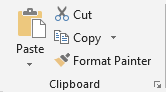
Cut/Copy/Paste - everyone knows these, and everyone uses these daily, in case someone doesn't know what Cut does, it copies the data by deleting it from it's original source, pasting it in the destination, in the end the user has the data only in the pasting destination, while the normal Copy keeps the data in both location (copying area and pasting destination)
Format Painter - a tool used to copy the style of the current Cell to another Cell, you can test it by applying background color on a cell, select the Format Painter tool and press a new cell, the new cell with have the same styles applied as the original cell
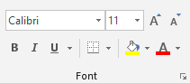
In the next column we have styles related to text, font type (name), size, styles (bold, italics, underline), border styles (the dropdown menu allows you to pick different types of borders), cell background color and text color.
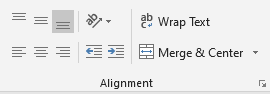
The following column is related to the text alignment, it allows you to align the text Top - Center - Bottom - Left - Middle - Right, allows you to add indentation, text wrapping and cell merging. The drop down arrow on Merge and Center gives you a couple more options, it's a small arrow and you might miss it.
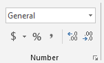
The next column we are checking is related to numbers mostly, here you can change the data types, maybe you need to use a date, or a currency, maybe something scientific, this is the area you are going to work with for these. You can see the menu allows you to add certain symbols and decimals if needed.
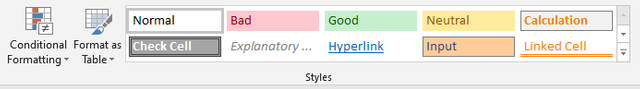
Our next stop is the Styles, here is the "fancy" part of our Spreadsheet. Let's start with conditional formatting, this allows you to change/format cells automatically using conditions. You set them as rules and will be applied to your rows/columns/cells.
Format as Table, here you can select an area of your spreadsheet and convert it to a specific table format presented in the menu, you have many premade examples, or you can create your own.
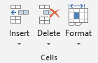
We are almost done, 2 more columns, next in line is the Cells column, here you can insert/delete columns or format them (increase/decrease height and width hide/unhide, autofit them based on the data inside)
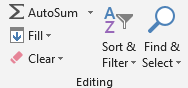
And the last one, the Editing one, here you can Sort and Filter data, Find specific data, replace it, validate it and many more.
Below all these, before hitting the spreadsheet itself we have 3 more tabs, first one is the navigation one, here you can write a specific Cell and while hitting enter, your cell selection will move to that specific Cell.
Then we have the formula insert, which inserts the formula in the next tab and prepares it for being used, the two buttons before the formula insert are used to apply or delete the formula selected.
After that we have the Spreadsheet itself with numbers applied on rows and letters on the columns.
Also did you know that if you zoom out enough, you can see the columns won't end after letter Z, the spreadsheet starts doubling the letters AA-AB-AC and so on, once it gets to AZ it changes the first letter and continues BA-BB-BC.
At the bottom we have the current sheet we are using, here you can rename it, or create a new one. Also on the bottom right side we have the zoom slider, something that you might need at one point :)
Second assignment
Based on the basic Formulas given in this lecture, use the data below to calculate the SUM Function and the AVERAGE Function of the class. Show clear working as to how you arrive at your answers.
Recreated the table in the Excel spreadsheet, also aligned it properly to keep the looks as real as possible, also prepared cells for the SUM and AVERAGE results.
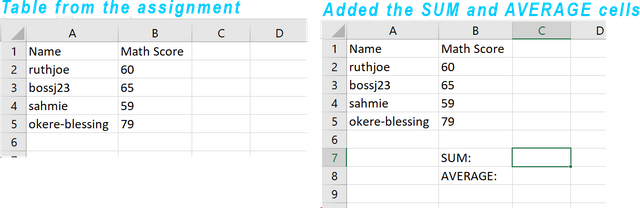
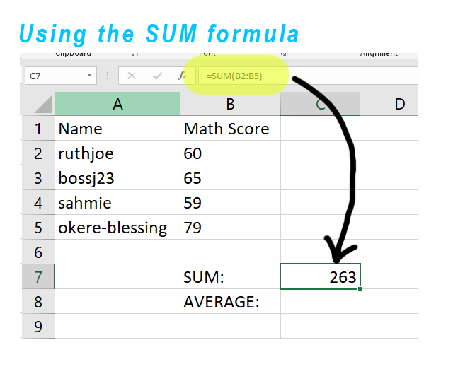
Using the SUM formula we've learnt in the course, we select the cell where we want the SUM value to be placed and we write the SUM formula in the formula's bar like this =SUM(B2:B5) which means, SUM of the values starting at position B2 until B5.
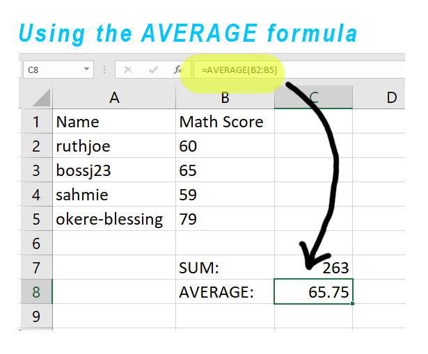
Using the same principle we use the AVERAGE formula, we move to the corresponding cell, where we want the AVERAGE result to be placed, and in the formula bar we write =AVERAGE(B2:B5).
The third assignment
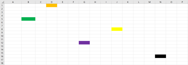
Take a screenshot of your worksheet and identify the cell Addresses of the following; N16 with a fill color of black, J8 with a fill color of yellow B5 with a fill color of Green G12 with a fill color of purple and D1 with a fill color of orange. Write your username on these cells using a visible font.
Now there are multiple ways to do this assignment, I'll show you two ways.
The first way is to use the name box left top corner, near the formula bar:
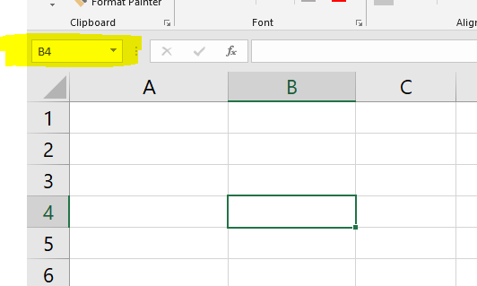
You write there the corresponding Cell you want to go to, press Enter and you are being moved to the desired cell.
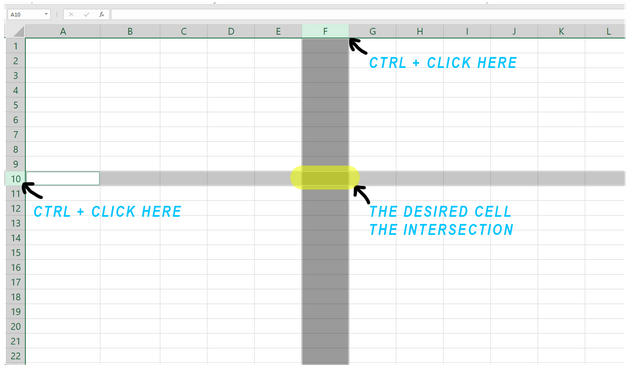
But you can also use CTRL + Click on the corresponding Row and Column, and the intersection of the selection will be the desired cell.
Now let's do the assignment, we are going to search for N16-J8-B5-G12-D1, 5 cells, 5 colors.
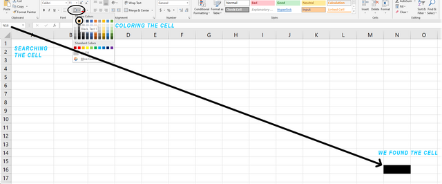
The steps are, we search the cell -> we find it -> we select it -> press the coloring tool -> select the proper color, and repeat these steps for all 5 cells required, in the end we get this.
The fourth and last assignment
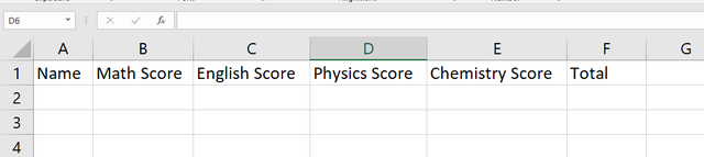
Prepare a score for 15 students where the cell A1 label will be Name, cell B1 label will be Maths Score, cell C1 label will be English Score, cell D1 label will be Physics Score, cell E1 label will be Chemistry Score and cell F1 will be labeled Total. Add all necessary information and calculate the total for each student. Show clear working.
We'll start by creating our work table, we start by adding the labels:
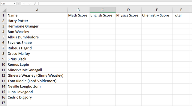
Time to add our students, a quick search on the google and we have the Harry Potter characters ready to take our classes.
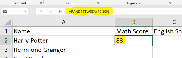
Now for the grades, we'll assume the lowest grade is 40 points, while the highest is 100, and because we've learnt about formulas, we are going to use the RANDOM BETWEEN formula to generate random scores between 40 and 100.
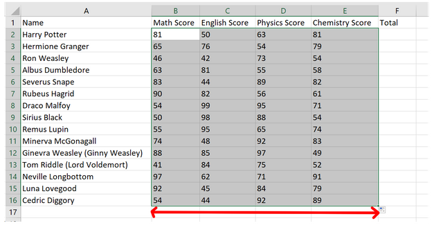
We have one cell that has it's random value, we can expand it to the whole column like this:

Click and hold the selection bottom right corner and drag it until you cover every student's grade cell and release the mouse after, the formula will be applied on every cell selected.
We can do these for the rows as well now, with the whole column selected, again hold the corner and cover all disciplines, like this:
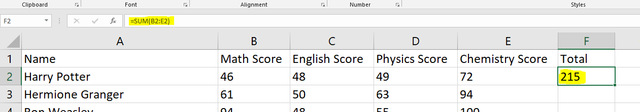
Now let's do the math and calculate the TOTAL for each student, we use the =SUM formula again, make sure we cover all the corresponding cells and we get the total. In our case it's from B2 to E2 to have all the disciplines taken into account.
Now, again we can expand the formula to all the Cells below and get the total for each student:
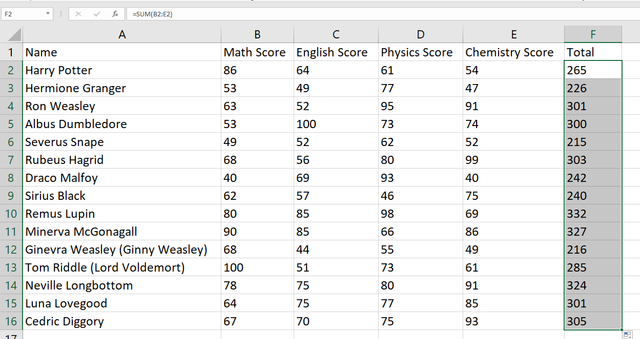
And here we have the total for each student.
Note: The numbers are different in each screenshot because while editing screenshots, I had to retake some steps and by this generating a new set of numbers.
That was it for this homework, it was fun, haven't used Excel since I was in middle school when we had Microsoft Office 2003 if I remember correctly.
I would also like to invite @titans @r0ssi @mojociocio to participate.
Thank you for this course @simonnwigwe and @josepha, can't wait to see the next part.
Also thank you reader for stopping by, wishing you all the best!
Thank you, friend!


I'm @steem.history, who is steem witness.
Thank you for witnessvoting for me.
please click it!
(Go to https://steemit.com/~witnesses and type fbslo at the bottom of the page)
The weight is reduced because of the lack of Voting Power. If you vote for me as a witness, you can get my little vote.
Thank you @josepha!
TEAM 4
Congratulations! Your post has been upvoted through steemcurator06. Good post here should be..Thank you @jyoti-thelight!
Es increíble la forma en la que nos ha explicado la composición de las hojas de cálculo, dónde se puede ubicar las funciones más importantes y el uso de las mismas, lo cual denota que tiene experiencia en el usod de estas herramientas.
Éxitos en el concurso.