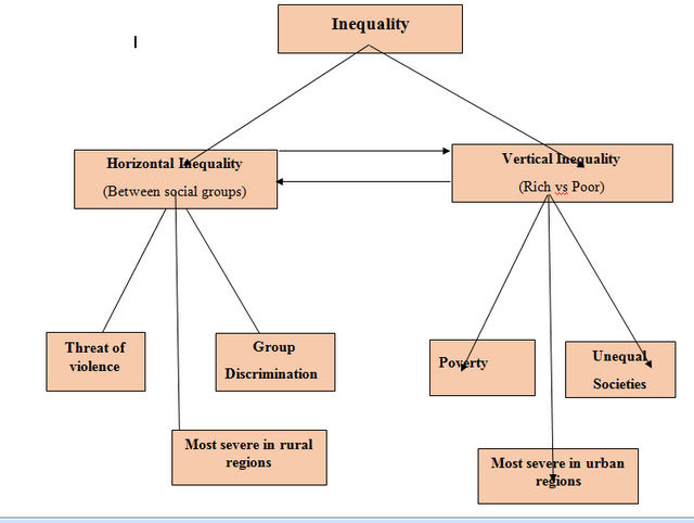
Economic inequality is defined as a difference found in various measures of economic well-being among individuals in a group, among groups in a population or among countries. Economic inequality is also refer as an income inequality, wealth gap or wealth inequality. Inequality means the unjust between different group of people when someone have more money, status or opportunities than others. Such difference of inequality may lead to polarization, feeling of exclusion from society and discrimination in a society. The whole world is fighting with inequality and other problems of extreme wealth. According to World Bank recent report, the growing global inequality crisis had led to just 62 people owing the same collective wealth as the poorest half of humanity. The global 1% now own more than everyone else combined.
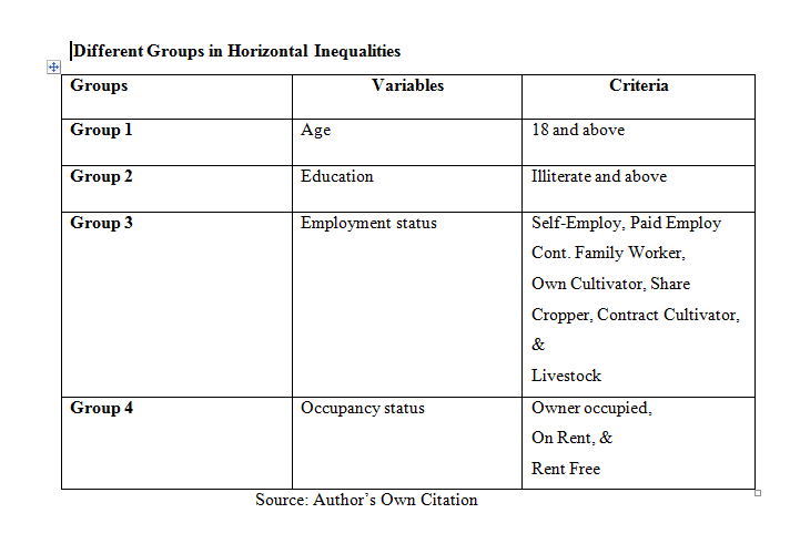
The major dimensions of horizontal inequalities are economic, political, social as well as cultural. These main dimensions included multiple elements which are given below
 Economic horizontal inequalities takes account of inequality of ownership or access of assets. Such as human, financial and natural resource based.
 Social horizontal inequalities takes account of inequality within inclusion of access, in service. Such as health care or status, housing and education.
 Political horizontal inequalities take account of inequality in distribution of power and opportunities among groups with the inclusion of control over army and police, national and provisional assemblies and the bureaucracy.
 Cultural horizontal inequalities take account of inequality among the different groups based on language, customs and demographic.

#RATIONALE OF THE STUDY
Pakistan has historically been a serious victim of vertical and horizontal inequalities. While findings vertical and horizontal inequalities, this study restricted to only Punjab and KPK province, mainly due to the following reasons. First, to best of researcher knowledge, the previous studies did not perform a comparative analysis of horizontal and vertical inequalities between two provinces of Pakistan (Punjab and KPK). Second, the population of Punjab and KPK are covering more than the population of other provinces. Third, there is a suspected higher variation in the degree of income inequality across the regions due to the importance of provincial capitals Lahore and Peshawar in terms of economic activities. Fourth, this is a cross sectional study to compare two province, if the study is restricted to only one province then panel data is feasible. Fifth, the researcher put it aside for future study and for researchers. In view of the chances of higher degree of inequality in Punjab and KPK province, this study specifically targeted the Punjab and KPK province.

#RESEARCH QUESTIONS
a) How does horizontal and vertical inequality initiates?
b) How much horizontal and vertical inequality persist in Punjab and KPK province?
c) How much income inequality prevails in urban and rural regions of Punjab and KPK province?
d) What are the best possible ways to handle horizontal and vertical inequality?#

#PURPOSE OF THE STUDY
The purpose of this study is to measure the horizontal inequality in overall Punjab and KPK. Vertical inequality is to be measured to analyze income inequality in Punjab and KPK divisions. Furthermore, the main purpose of the objective is to compare the horizontal or vertical inequality between Punjab and KPK.

#FOCUS OF THE STUDY
The main focus of this study is to check either horizontal or vertical inequalities harms the economy of Pakistan. All appropriate index are used for the empirical analysis of the Punjab and KPK. At last, a comparative analysis of both the provinces are conducted.

#OBJECTIVES OF THE STUDY
a) To estimate horizontal inequalities in overall Punjab and KPK.
b) To perform comparative analysis of horizontal inequalities between Punjab and KPK.
c) To estimate income inequalities (vertical inequalities) in Punjab and KPK at divisional level.
d) To perform comparative analysis of vertical inequalities between Punjab and KPK

The basic #aim of the study is to perform the comparative analysis of horizontal income inequality between KPK and Punjab. For this study, a secondary data set is being used to measure the horizontal and vertical inequality namely Household Integrated Economic Survey (HIES) for the year 2015-16, which is being collected by Pakistan Bureau of Statistics (PBS). PBS has the duty to conduct the survey for the collection of the data from sampled household which represents the population. The survey provides information about all the provinces of Pakistan at National and Provincial level including rural and urban regions.
The #HIES, Household Income and Expenditure Survey dataset provides data and information about all the provinces of Pakistan including rural and urban areas. The data and information about those areas which are under the control of forces of Pakistan are not included in the survey because of confidentiality. Furthermore, due to policy restrictions, the data and information of AJ&K, Gilgit Baltistan and FATA, Federally Administrated Tribal Areas did not release by the government.

#Sampling Framework
PBS, Pakistan Bureau of Statistic has maintained its own sampling technique for rural and urban domain. In which every town or city is divided into enumeration blocks. Each block has a well-defined boundaries which comprised of an average 200 to 250 households.

#Sample Design
PBS, Pakistan Bureau of Statistic adopted a stratified two-stage sample design for the survey.
#Sample size and its Allocation
The sample size consist of 26688 households for the four provinces which is distributed over 1668 PSU’s, out of which 1115 are urban and 553 are rural. This sample size is considered to be an appropriate sample size which provide a consistent estimation for the four provinces at provincial level with rural and urban breakdown. Nevertheless, this dataset covering 24238 households by collecting data from 1605 PSU’s. Due to bad law and order situation 63 PSU’s (35 rural and 28 urban) were dropped.

#DATA RELATED ASSUMPTION
Assumption for using household aggregate consumption expenditure as an income proxy is that income component responses in the survey are considered less reliable than consumption items. This is because to avoid tax, the inadequacy of agricultural markets, the more impulsive nature of rural income, and the incidence of large non-monetized rural transactions. Consumption expenditure on non-durable goods are considered in the study as a more reliable proxy for income.

#WHY CHOOSING DIFFERENT INEQUALITY INDEXES?
To capture different dimensions of inequality a single index is not suitable. All indexes focuses on different dimensions of inequality and vary in their properties. The main idea behind selection of indexes depend on the type of research question and hypothesis which are going to be tested. Before selection of any indexes it is necessary to focus on the dimensions which are going to be measured and select the indexes which satisfies the requirement of study
So different approaches such as Gini Coefficient, Atkinson’s Index and Generalized Entropy measure are used to measure horizontal and vertical inequalities in Punjab and KPK. Detail of different indexes are as follows.

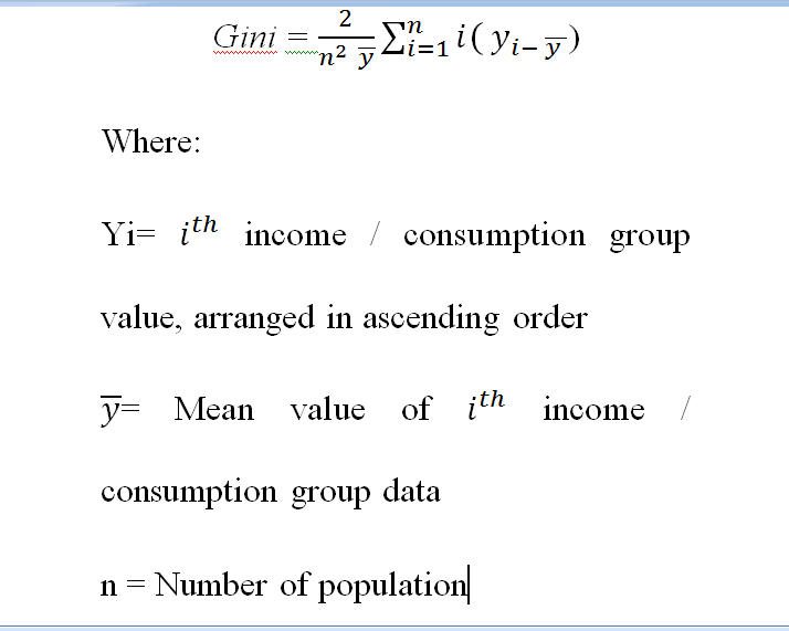
#Gini Coefficient
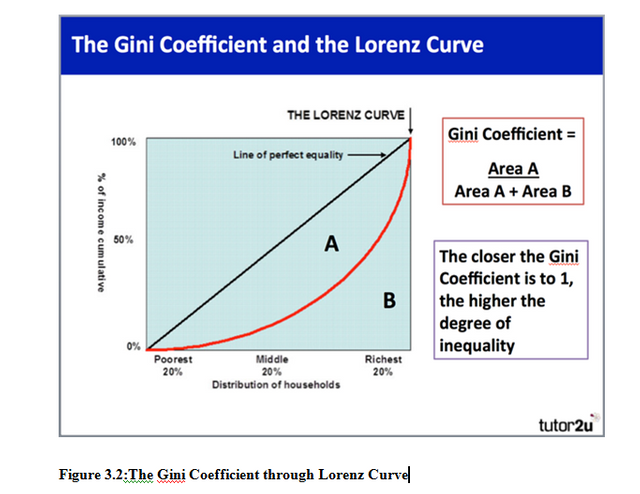
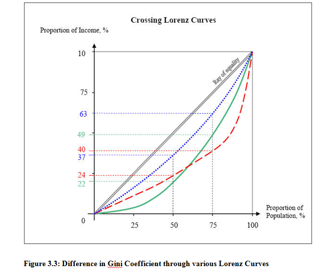
Gini Coefficient is the most commonly used measure of inequality by the researcher. Gini Coefficient is based on the Lorenz Curve which shows the distribution of income. The Lorenz curve is derived by taking the cumulative percentage of population on x-axis and cumulative percentage of income on y-axis. The perfect line of equality i.e. 45° shows an equal distribution of income. The kinked Lorenz Curve shows an unequal distribution of income i.e. the more kinked curve the more unequal distribution of income. Gini coefficient can also be measured by a formula Area A/ Area (A + B). This formula shows that if A=0 than Gini coefficient will be 0 and it shows a perfect equality and if B=0 than Gini coefficient will be 1 and it shows a perfect inequality.

#Limitations of Gini coefficient:
Issue 1: Gini coefficient cannot tell us anything regarding the income share of particular quintile.
Issue 2: Lack of information towards different parts of distribution. In figure 3.2, crossing of Lorenz curves does not justify redistributive policies.
Issue 3: The Gini coefficient does not satisfies decomposability criteria or additive across groups.

#Which indexes satisfy these issues?
The World Bank Group (2005) and Stewart et al., (2005) provided a number of alternative indexes which does not suffer from the above mentioned issues:
Theil’s Index
Atkinson’s Index
Both of these indexes fulfill the criteria of decomposability. They decomposed by income factor or partition group. Theil index is decomposed at 0 and 1 for the parameter α. Similarly, Atkinson’s Index is decomposed at 0.5, 1 and 2. Detail of these indexes is as under.

Generalized Entropy Measures

Generalized entropy measures are another alternative approach used by many researchers to overcome the issues of Gini coefficient. This approach is further divided into two methods: Theil indexes and mean log deviation measure. Both belonged to a family of generalized entropy measures. By assuming the social welfare function as a natural logarithm the generalized entropy index can be converted into a subclass of Atkinson index. Generalized entropy index has a unique class which satisfy the property of decomposability. The general formula for entropy measure is,

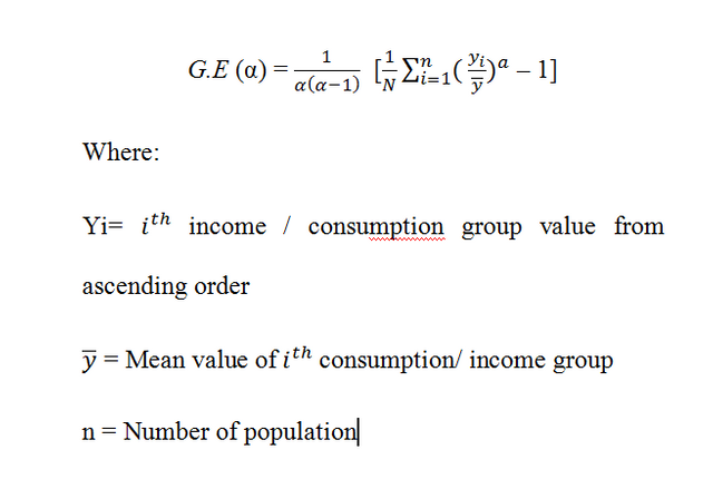
The values Generalized Entropy measures vary between 0 and 1, where zero shows an equality and higher value shows higher level of inequality.
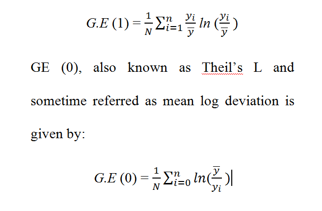
The parameter α represents the weigh given to distance between incomes at different parts of the income distribution. For lower value of α, generalized entropy is more sensitive to lower tail of the distribution and for higher valuesof αgeneralized entropy is more sensitive to the upper tail. Most commonly used values of αare 0, 1 and 2, where GE (0) is mean log deviation, GE(1) is the Theil’s T index and GE(2) is coefficient of variation.

Theil (1967) formulated two inequality indexes from the entropy measures. G.E (1) is Theil’ T index having a formula as,

#Atkinson’s Inequality Measure
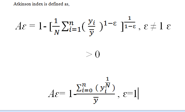
The World Bank Group (2005) and Stewart et al., (2005) also suggested another class of inequality measure that are used by many researchers.Atkinson formulated another inequality index by imposing weighted coefficient ԑ to incomes. The Atkinson coefficient ԑ is also known as ‘inequality aversion parameter’. The coefficient tells the amount of social utility gained by redistribution of resources. For ԑ = 0, it is assumed that by redistributing resources there is no social utility gained so no aversion to inequality. For ԑ = ∞, it is assumed that by distributing resources there is an infinite social utility gained so infinite aversion to inequality. Thus lower value of Atkinson index Aԑ indicate low gained from social utility, higher value of Aԑ indicate high gained from social utility.
Atkinson index is defined as,

#HOUSEHOLD IN PUNJAB AND KPK
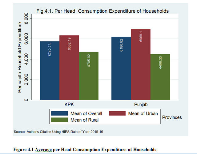
Figure 4.1 shows the average per head consumption expenditure of household in province Punjab and KPK along with representative rural urban region. Estimated figure shows that at provincial as well as region level household of Punjab have higher consumption expenditure as compared to their counterpart. In province Punjab, average estimated expenditure of households are 6186.82 rupee per month while in KPK such expenditures are 5742.73 rupee per month. Similarly, at regional level urban estimates are 6969.1 rupee per month in Punjab and 6332.19 rupee per month in KPK while rural estimates of both province are 4498.35 and 4705.2 rupee per month respectively.

#RESULTS OF DIVISIONAL BASED VERTICAL INEQUALITIES
Vertical inequalities is defined as inequality measure among individuals or households. Vertical inequalities is important because an equal society have more happiness than unequal society and an equal society grow faster than an unequal society.
#Divisional Estimates of Vertical Inequality in Province Punjab#
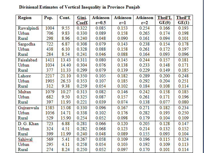
As shown below in Table demonstrates the divisional measure of inequality in province Punjab along with representative rural urban region of each division. Current study has used per head consumption expenditure as a proxy of per head income to investigate the extent of problem in each division and its representative region.
Estimated outcomes of province Punjab demonstrate that 34.10 percent inequality exist in overall province with urban and rural measurement 34.40 and 27.30 percent. Similarly, Atkinson measure of inequality shows the overall inequality in province Punjab and its rural urban regions with varying epsilon value 0.5, 1,2 are 9.80, 17.30, 28.10; 9.90, 17.50, 28.50 and 6.20,11.40 and 19.70 percent respectively, which demonstrate that varying value of epsilon in Atkinson is more sensitive to inequalities in the lower income distribution. However, in case of Theil’L and Theil’T estimated results for given division with urban and rural regions are 18.70, 22.90; 19.30, 23.20, 12.10 and 13.80 percent respectively which also clarify that the sensitivity parameter theta is more sensitive to inequalities at the top of the income distribution.
Similar to above discussion, estimated outcomes of all the divisions like Rawalpindi, Sargodha, Faisalabad, Lahore, Multan, Gujranwala, D.G. Khan, Sahiwal, Bahawalpur and Federal areas Islamabad demonstrate that inequality has similar trend in all measures especially the estimates of Atkinson and Theil’s measures suggest that with varying value of both epsilon and theta given rise to inequality which concludes that both inequality measure are much sensitive toward bottom and top income group. While overall discussion signifies that Islamabad is facing high income/consumption inequality in all three measures while opposite is true for Sahiwal division because in Islamabad division, per head consumption expenditure of household are high as compared to all division while Sahiwal division has lower per head consumption expenditure.

#Divisional Estimates of Vertical Inequality in Province KPK#
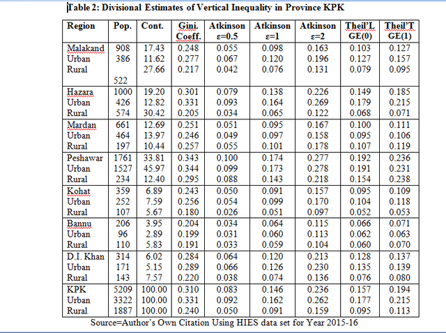
Table 2 validates the divisional outcomes of inequality in province KPK along with demonstrative rural urban region of each division. Current study has used per head consumption expenditure as a proxy of per head income to examine the extent of problem in each division and its descriptive region.
Estimated outcomes of province KPK demonstrate that 31.10 percent inequality exist in overall province with urban and rural measurement 33.10 and 24.10 percent. Similarly Atkinson measure of inequality shows the overall inequalityin Province KPK and its rural urban regions with varying epsilon value 0.5, 1,2 are 8.30, 14.60, 23.60; 9.20, 16.20, 26.20 and 5.00,9.10 and 15.90 percent respectively, which demonstrate that varying value of epsilon in Atkinson is more sensitive to inequalities in the lower income distribution. However, in case of Theil’L and Theil’T estimated results for given division with urban, rural regions are 15.70, 19.40; 17.70, 21.50, 9.50 and 11.30 percent respectively, which also explain that the sensitivity parameter theta is more sensitive to inequalities at the top of the income distribution.
Similar to above discussion, estimated outcomes of all the divisions like Malakand, Hazara, Mardan, Peshawar, Kohat, Bannu and D.I.Khan demonstrate that inequality has similar trend in all measures especially the estimates of Atkinson and Theil’s measures suggest that with varying value of both epsilon and theta given rise to inequality which concludes that both inequality measure are much sensitive toward bottom and top income group. While overall discussion signifies that Peshawar division is facing high income/consumption inequality in all three measures while opposite is true for Bannu division because in Peshawar per head consumption expenditure of household are high as compared to all division while Bannu has lower per head consumption expenditure.

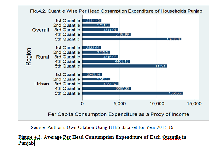
#AVERAGE PER HEAD CONSUMPTION EXPENDITURE OF EACH QUANTILE IN PUNJAB AND KPK
Figure 4.2 shows the average per head consumption expenditure of household in five quantile of Punjab and its representative rural and urban regions. Calculation of Punjab shows 1st quantile have lowest per head consumption expenditure i.e. 2584.2 rupee while 5th quantile shows highest per head consumption expenditure of 13296.9 rupee. Estimated measures of overall Punjab shows that with varying quantile from 1 to 5 per head consumption expenditure increased and estimated figure concludes that 1st quantile belong to a group having lowest 20 percent consumption expenditure while last quantile having upper class households with highest per head consumption expenditure. Similar estimates have been shown for both region while all the quantile of urban region reveals that households of such region have higher per head consumption expenditure and better living standard as compared to their counterparts.
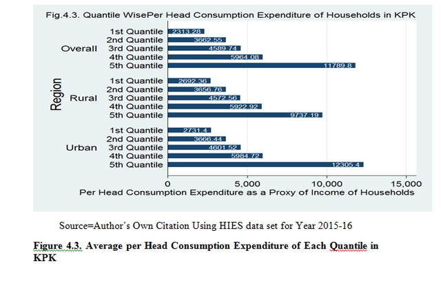
Likewise above discussion figure 4.3 demonstrates the per head consumption expenditure of household in province KPK and its region in all five quantile. Calculated results of overall province shows the increase in per head consumption expenditure from 1st quantile to 5th quantile. Initial quantile has per head consumption expenditure of households 2313.28 rupee per head while last quantile have 11789.8 rupee. Estimated results shows that initial quantile represents the consumption expenditure of lowest 20 percent while 5th quantile shows top 20 percent consumption expenditure. Similarly, regional estimates states that at each quantile households of urban region has higher per head consumption expenditure and better standard of living as compared to its complement.

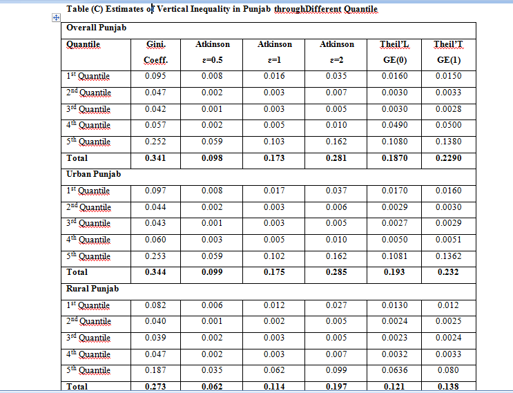
#Inequality Estimates of Province Punjab through Different Quantile
Table (C) reports the measurement of vertical inequality in province Punjab along with representative urban rural region through different quantile. Estimated results of all five quantile shows that due to minor difference in per head consumption expenditure of households first four quantile show little bit fluctuation in inequality while household in quantile five have higher per head consumption expenditure and also have higher inequality across all measure like Gini coefficient , Atkinson and Theil’s measure. Results of 5th quantile reveals that there exist 25.20 percent inequality among the household while estimates of Atkinson measure along with varying epsilon 0.5, 1 and 2 reports that inequality increase from 5.90, 10.30 and 16.90 percent respectively, which demonstrate that varying value of epsilon in Atkinson is more sensitive to inequalities in the lower income distribution. Likewise Atkinson estimates results of Generalized Entropy Index also shows similar pattern and reveal that varying value of theta 0 and 1 inequality increase from 10.80 to 13.50 percent which conclude that the sensitivity parameter theta is more sensitive to inequalities at the top of the income distribution. Similar trend has been presented by both urban and rural region of given province where inequality is significant higher in 5th quantile as compared to all other quantile of both regions. In case of urban areas, due to modernization and higher consumption expenditure inequality is higher in all quantile as compared to their rural counterpart while Atkinson and Theil’s measure suggested that epsilon and theta are more sensitive toward inequality at bottom and top income distribution.

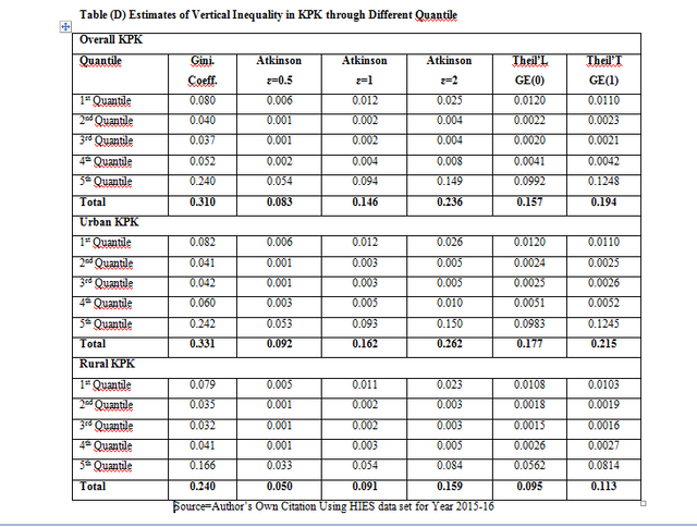
#Inequality Estimates of Province KPK through Different Quantile
Table (D) reveals the inequality estimates of province KPK along with representative rural and urban region through different quantile. Calculated results of the all the quantile for overall province shows that from quantile 1 to 4 inequality is not much higher and also presenting same measure with little bit fluctuation because of minor difference in per head consumption expenditure of the households while 5th quantile reveals a clear difference of per head consumption expenditure of household and also inequality. All the measures of inequality exposed that due to upper class in 5th quantile inequality is higher with Gini-coefficient measure 24 percent .Atkinson results along with varying epsilon 0.5,1 are 5.4, 9.4 and 14.90 percent. Generalized Entropy Index showing estimates of Theil’L and Theil’T with varying theta are 9.92 and 12.48 percent respectively. Similar to above discussion, with varying value of epsilon and theta inequality rise which conclude that Atkinson and Theil’s measures are more sensitive toward income inequality in lower and upper income distribution. Similar trend has been presented by both urban and rural region of given province where inequality is significant higher in 5th quantile as compared to all other quantile of both regions. In case of urban areas due to modernization and higher consumption expenditure inequality is higher in all quantile as compared to their rural counterpart while Atkinsonand Theil’s measure suggest that epsilon and theta are more sensitive toward inequality at bottom and top income distribution.
Comparative study of both province reveals that at each step per head consumption expenditure and inequality is higher in province Punjab as compared to KPK because in province Punjab most of the households belong to urban areas and have clear difference in their earning while in KPK expect few division, most of the household belong rural areas and attach with same earning activity like agriculture therefore their expenditure have very little fluctuation and have lower inequality.
RESULT OF HORIZONTAL INEQUALITY IN OVERALL PUNJAB & KPK
Horizontal inequalities defined as inequality measure among groups i.e. religious, cast, sect, cultural, political, education, gender, age, and employment based groups. Horizontal inequality is important because it leads to violent conflict. Furthermore, it is important because vertical inequality is restricted to only few economic variable whereas horizontal inequality goes beyond those variable as it also includes social and political variables.

#Horizontal Inequality through Different Age Groups of Punjab
Horizontal inequality estimates for province Punjab through different age groups in table (A) reveals that the household head having age from 18 to 30 have income/consumption inequality 33.40 percent with Atkinson and Theil’s estimates 9.30,16.60 and 27.30; 18.10 and 21.50 percent. Estimates of given age group demonstrates that with varying value of epsilon and theta Atkinson and Theil are more sensitive to lower and bottom income/consumption group in current segment of the study. Estimates of all age groups reveal similar trend in description like initial one while elder household who are living by utilizing transfer payment or pension allowances are facing higher consumption inequality with estimates of gini- coefficient 38.70 percent with Atkinson and Theil’s calculation 12.70, 21.60 and 33.30; 24.40 and 30.30 percent. However, comparative study of different age group concludes that age group 31-40 years has smaller inequality estimates because household head in such age are mostly employed and expect few mostly attached with similar consumption pattern while age group consists of elder households have higher income/consumption inequality.
The reason behind higher inequality in last group is that such group household’s head after leaving labor force become unemployed or relying on transfer payment which cause large difference in their consumption expenditure. Likewise above, urban estimates of inequality among same group present similar trend to overall province measures while rural region show significant fluctuations. Estimates of rural area demonstrates that higher inequality exist in 41-50 and lower exists in 31-40 while overall compression rural area showing smaller inequality as compared to their urban counterpart which concludes that due to modernization and different employment activities cause significant difference in inequality between two region while rural areas households mostly attached with agriculture and have similar crop growing pattern and living standard therefore such households facing lower income/consumption inequalities.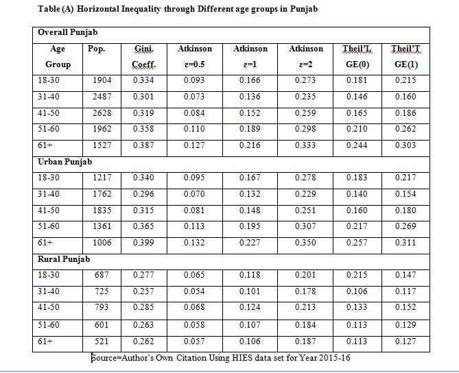

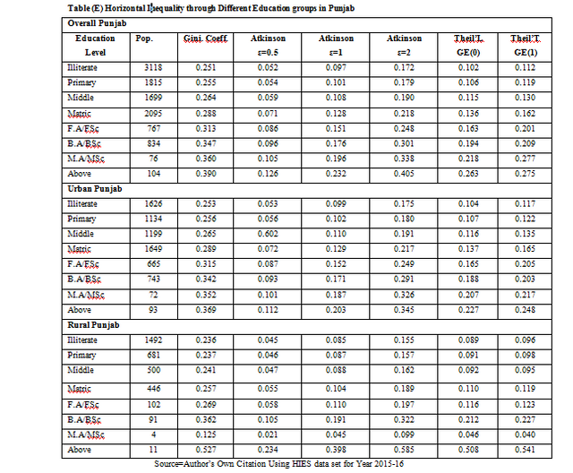
#Horizontal Inequality through Different Education Groups of Punjab
Table (E) estimates represents the results of horizontal inequality among different education groups. Calculated results shows that with increase in education level from illiterate to maximum education, inequality increases. Estimates of initial measure signifies that household head who are illiterate have smaller income/consumption inequality because mostly such households are attached with similar earning pattern and their income are just enough to meet minimum threshold that is necessary for normal standard of living. Estimated measure for such educational group indicates that inequality through Gini-coefficient is 25.10 percent with Atkinson and Theil’s calculation 5.2, 9.7 and 17.20; 10.2 and 11.20 which suggest that varying value of both epsilon and theta, Atkinson and Theil’s are more sensitive to bottom and top income distribution. Similarly varying educational years cause higher inequality which concludes that with varying education of household head cause higher earning income or earning opportunities which cause income inequality rise because most of the households with varying income of household head having little family size as compared to other households in a same group change their life style and moves toward luxuries life which cause the wider inequalities. Like preceding discussion of overall Punjab for current group, results of urban and rural region also reveal similar trend while increasing education in rural sector have smaller inequality effect as compared to urban counterpart except last measure in rural sector because in rural sector higher educated population is very small and have higher standard of living which cause significant income and consumption inequality among the households of such educational group. However, the calculated results of Gini-coefficient is 52.70 percent with Atkinson and Theil’s calculation 23.40, 39.80 and 58.50; 50.80 and 54.10 which suggest that varying value of both epsilon and theta, Atkinson and Theil’s are more sensitive to bottom and top income distribution.

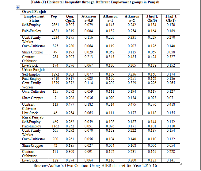
#Horizontal Inequality through Different Employment Groups of Punjab
Table (F) shows results of horizontal inequality for employment status discuss that household head who are self-employed have consumption inequality 30.70 percent with Atkinson and Theil’s estimates along with varying epsilon and theta are 7.90, 14.30 and 24.2; 15.40 and 17.80 percent respectively. Similarly, estimates of paid employed reveals that consumption inequality is 31.90 percent with Atkinson and Theil’s estimates 8.40, 15.20, 24.40; 16.40 and 18.90 percent which suggest that varying value of both epsilon and theta Atkinson and Theil’s are more sensitive to bottom and top income distribution. Like preceding discussion households related to different professions have different inequality estimates while households related to the profession of share cropper have smaller inequality with estimated measure 19.30; 2.9, 5.80, 11.50; 5.90 and 5.58 percent respectively. However, household who are contract cultivator have higher consumption inequality with estimated measure 37.5; 11.60, 20.50, 33.10; 22.90 and 27.00 percent respectively. In case of regional estimates, similar trend has been shown by both urban and rural region while at every position rural inequality estimates are smaller than urban complement which concludes that rural areas household having different occupation does not affect their life style and leading such life style which is quite closer to each other but basic reason of inequality among these household is because of educational difference and some big guns living in rural areas.

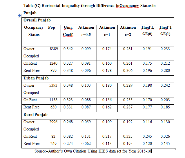
#Horizontal Inequality through Different Occupancy Status Groups of Punjab
Occupancy status estimates for horizontal inequality in table (G) for Punjab reveal that households who are living rent free have higher consumption inequality with estimated measure of Gini-coefficient 34.80 percent, Atkinson estimates with varying epsilon are 9.60, 17.80 and 30.6 percent and Theil’s estimates with varying theta are 19.60 and 28.00 percent. However estimates of owner occupied suggest that 34.20 percent inequality exist among households through Gini-coefficient while Atkinson estimates along with varying epsilon and Theil’s measure along with varying theta are 9.90, 17.40 and 28.10; 19.10 and 23.33 percent. Similar to preceding discussion results of household on rent describes that 32.70 percent inequality exist among them through Gini- coefficient while estimates of Atkinson and Theil’s reveals that with fluctuating value of epsilon and theta inequality increase and measures are 9.10, 16.00 and 26.10; 17.50 and 21.20 percent respectively. Overall estimates of Atkinson and Theil measure shows that varying value of epsilon and theta increase inequality in all three groups which concludes that Atkinson and Theil’s are more sensitive to bottom and top income distribution. In case of urban results, households who are owner occupied facing higher inequality as compared to other and in case of rural segment households who are on rent are facing higher consumption inequality. Comparative analysis shows that except on rent in rural areas urban households have higher inequality in all the groups because as compared to rural households urban sector have better living standard and due to modernization households of urban areas strong stretched toward demonstration effect which cause serious inequality among them.

#Horizontal Inequality through Different Age Groups of KPK
Horizontal inequality estimates for province KPK through different age groups in table (H) reveal that the household head having age from 18 to 30 have income/consumption inequality 29.40 percent with Atkinson and Theil’s estimates 7.90,13.50 and 21.80; 14.60 and 19.20 percent. Estimates of given age group demonstrates that Atkinson’s and Theil’s indexes are more sensitive to lower and bottom income/consumption group in current segment of the study. Estimates of all age groups reveal similar trend in description like initial one while elder household who are living by utilizing transfer payment or pension allowances are facing higher consumption inequality with estimates of Gini- coefficient 36.00 percent with Atkinson and Theil’s calculation 11.30, 19.10 and 29.40; 21.20 and 27.40 percent. However, comparative study of different age group concludes that age group 31-40 has smaller inequality estimates because household head in such age are mostly employed and expect few mostly attached with similar consumption pattern while age group consists of elder households have higher income/consumption inequality. The reason behind higher inequality in last group is that such group household’s head after leaving labor force become unemployed or relying on transfer payment which cause large difference in their consumption expenditure. Likewise above, urban estimates of inequality among same group present similar trend to overall province measures while rural region show significant fluctuations. Estimates of rural area demonstrates that higher inequality exist in 61+ and lower exists in 18- to 30 while overall compression rural area showing smaller inequality as compared to their urban counterpart which concludes that due to modernization and different employment activities cause significant difference in inequality between two region while rural areas households facing lower income inequalities because mostly 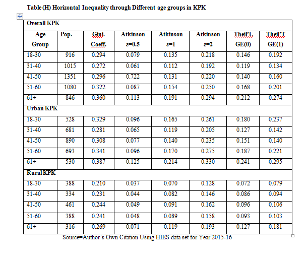households attached with agriculture and have similar living standard.

#Horizontal Inequality through Different Education Groups of KPK
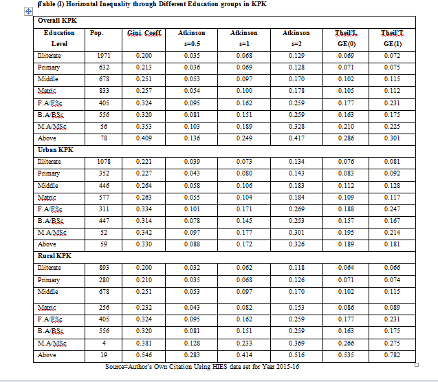
Table (I) estimates represents the results of horizontal inequality among different education groups in province KPK. Calculated results shows that with increase in education level from illiterate to maximum education inequality increases. Estimates of initial measure signifies that household head who are illiterate have smaller income/consumption inequality because mostly such households are attached with similar earning pattern and their income are just enough to meet minimum threshold that is necessary for normal standard of living. Estimated measure for such educational group indicates that inequality through Gini-coefficient is 20.00 percent with Atkinson and Theil’s calculation 3.50, 6.8 and 12.90; 6.90 and 7.20 which suggest that varying value of both epsilon and theta, Atkinson and Theil’s are more sensitive to bottom and top income distribution. Similarly varying educational years cause higher inequality which concludes that with varying education of household head lead to higher earning income and earning opportunities which cause income inequality rise. Another reason is that households with varying income of household head having little family size as compared to other households in a same group change their life style and moves toward luxuries life which cause the wider inequalities. Like preceding discussion of overall KPK for current group, results of urban and rural region also reveal similar trend while increasing education in rural sector have smaller inequality effect as compared to urban counterpart except last measure in rural sector because in rural sector higher educated population is very small and have higher standard of living which cause significant income and consumption inequality among the households of such educational group. However, the calculated results of Gini-coefficient is 54.60 percent with Atkinson and Theil’s calculation 28.30, 41.40 and 51.16; 53.50 and 78.20 which suggest that varying value of both epsilon and theta, Atkinson and Theil’s are more sensitive to bottom and top income distribution

#Horizontal Inequality through Different Employment Groups of KPK
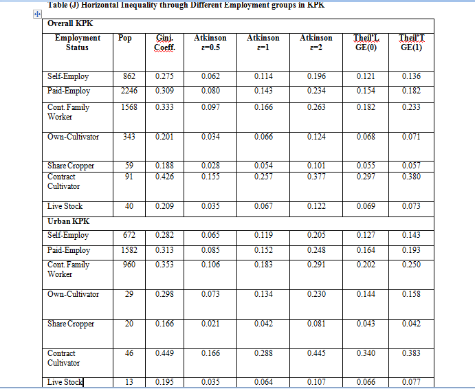
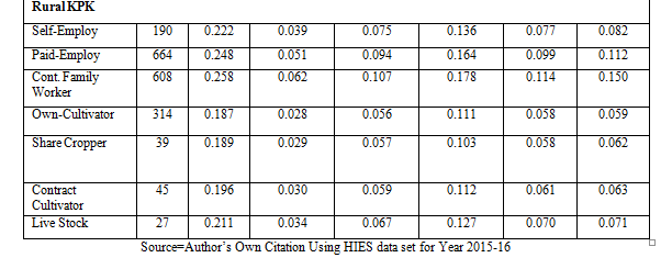
Table (J) results of horizontal inequality for employment status discuss that household head who are self-employed have consumption inequality 27.50 percent with Atkinson and Theil’s estimates along with varying epsilon and theta are 6.20, 11.40 and 19.60; 12.10 and 13.60 percent respectively. Similarly, estimates of paid employed reveals that consumption inequality is 30.90 percent with Atkinson and Theil’s estimates 8.00, 14.30, 23.40; 15.40 and 18.2 percent which suggest that varying value of both epsilon and theta, Atkinson and Theil’s are more sensitive to bottom and top income distribution. Like preceding discussion, households related to different professions have different inequality estimates while households related to the profession of share cropper have smaller inequality with estimated measure 18.80; 2.8, 5.40, 10.10; 5.50 and 5.70 percent respectively. However, household who are contract cultivator have higher consumption inequality with estimated measure 42.60; 15.50, 25.70, 37.70; 29.7 and 38.00 percent respectively. In case of regional estimates similar trend has been shown by both urban and rural region while at every position rural inequality estimates are smaller than urban complement which concludes that rural areas household having different occupation does not affect their life style and leading such life style which is quite closer to each other but basic reason of inequality among these household is because of educational difference and some big guns living in rural areas.

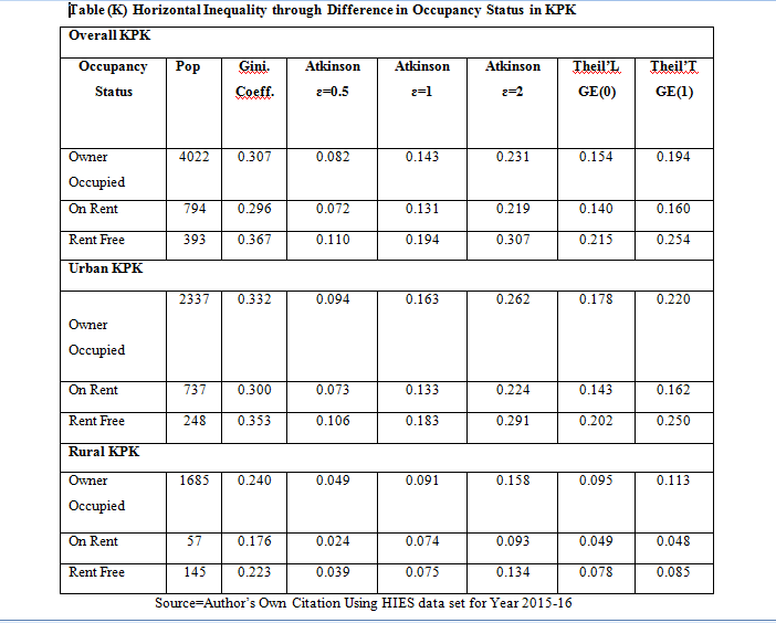
#Horizontal Inequality through Different Occupancy Status Groups of KPK
Occupancy status estimates for horizontal inequality in table (K) for KPK reveals that households who are living rent free have higher consumption inequality with estimated measure of Gini-coefficient 36.70 percent, Atkinson estimates with varying epsilon are 11.00, 19.40 and 30.70 percent and Theil’s estimates with varying theta are 21.50 and 25.40 percent. However, estimates of owner occupied suggest that 30.70 percent inequality exist among households through Gini-coefficient while Atkinson estimates along with varying epsilon and Theil’s measure along with varying theta are 8.20, 14.30 and 23.10; 15.40 and 19.40 percent. Similar to preceding discussion, results of household on rent describes that 29.60 percent inequality exist among them through Gini- coefficient while estimates of Atkinson and Theil’s reveals that with fluctuating value of epsilon and theta inequality increase and measures are 7.20, 13.10 and 21.90; 14.00 and 16.00 percent respectively. Overall estimates of Atkinson and Theil measure shows that varying value of epsilon and theta increase inequality in all three groups which concludes that Atkinson and Theil’s are more sensitive to bottom and top income distribution. In case of urban region, results households who are rent free facing higher inequality as compared to other and in case of rural segment, households who are owner occupied are facing higher consumption inequality. Comparative analysis shows that urban households have higher inequality in all the groups as compared to rural households because urban sector have better living standard and due to modernization households of urban areas strong stretched toward demonstration effect which cause serious inequality among them.

#SUMMARY
The study investigates the horizontal and vertical inequalities at overall and divisional level of the province Punjab and KPK along with rural and urban regions. Different inequality measures provided by the World Bank group (2005) are adopted to measure inequality such as Gini coefficient, Theil’L, Theil’T and Atkinson’s Index by using the micro data set namely Household Income and Expenditure Survey (HIES) for the period 2015-16.
It is to be found by using all indexes thatPunjab is facing 34.10 percent income inequality in overall province with urban and rural measurement 34.40 and 27.30 percent. At divisional level estimates, the results show that Islamabad division is facing high income inequality with Gini coefficient 39.3 percent with urban and rural measurement 38.2 and 44.1 percent while Sahiwal division is facing low income inequality with a Gini coefficient 26.7 percent with urban and rural measurement 25.8 and 25.50 percent. According to Gini coefficient, ranking of income inequality in different divisions of Punjab is as follows, Islamabad with 39.3 percent, Lahore with 35.0 percent, Gujranwala with 33.0 percent, Bahawalpur with 32.30 percent, Rawalpindi with 32.20 percent, Multan with 31.30 percent, Faisalabad with 31.10 percent, Sargodha with 30.80 percent, D.G Khan with 28.10 percent and Sahiwal with 26.70 percent. Furthermore, the province KPK is facing 32.10 percent income inequality in overall province with urban and rural measurement 33.1 and 24.0 percent. At divisional level estimates, the results show that Peshawar division is facing high income inequality with Gini coefficient 34.3 percent with urban and rural measurement 34.4 and 29.5 percent whereas Bannu division is facing low income inequality with Gini coefficient 20.4 percent with urban and rural measurement 19.9 and 19.1 percent. According to Gini index, ranking of income inequality in different divisions of KPK is as follows, Peshawar with 34.30 percent, Hazara with 30.10 percent, D.I.Khan with 28.40 percent, Mardan with 25.10 percent, Malakand with 24.80 percent, Kohat with 24.30 percent and Bannu with 20.40 percent. The comparative analysis shows that Punjab is facing higher income inequality than KPK. Similarly at divisional level, Punjab’s divisions are also facing more income inequalities than KPK’s divisions. The capital of Punjab, Islamabad division is facing 39.30 percent income inequality whereas the capital of KPK, Peshawar division is facing 34.30 percent income inequality. Furthermore, estimates of horizontal inequalities at overall Punjab through different groups show that first group (age group) 61+ years are facing high inequality withGini coefficient 38.70 percent whereas the age group 31-40 years is facing low inequality with Gini coefficient 30.10 percent. Atkinson and Theil index with varying epsilon and theta also shows the similar results. The horizontal inequality at overall Punjab through second group shows that people with higher education level face higher inequality with Gini coefficient estimate 39.0 percent with urban and rural measurement 36.90 and 52.70 percent respectively, whereas people with no education face low inequality with Gini coefficient 25.1 percent. The urban region shows the similar results but rural region shows some fluctuations.The horizontal inequality at overall Punjab through third group shows that people who are contract cultivator face higher inequality with Gini coefficient 50.70 percent with urban and rural measurement 47.70 and 30.90 percent respectively whereas households related to a profession of share cropper face low inequality with Gini coefficient 19.30 percent with urban and rural measurement 20.80 and 18.50 percent. All other indexes also show the similar results. The horizontal inequality at overall Punjab through fourth group shows that households who are living rent free face higher inequality with Gini coefficient 34.80 percent but Atkinson index with parameter 0.5 shows higher inequality among owner occupied group whereas households who are on rent face low inequality with Gini coefficient 32.70 percent.In case of urban, results show that households who are owner occupied facing higher inequality with Gini coefficient 34.80 percent as compared to other and in case of rural segment households who are on rent facing higher consumption inequality with Gini coefficient 38.20 percent. Furthermore, the horizontal inequality at overall KPK through different groups show that first group (age group) 61+ years face high inequality with Gini coefficient 36.0 percent whereas age group 31-40 years face low inequality with Gini coefficient 27.20 percent respectively. The urban estimates of inequality among same group present similar trend to overall province measures while rural region show significant fluctuations. The horizontal inequality at overall KPK through second group shows that with increase in education level from illiterate to maximum education inequality increases. The estimates show that household head who is illiterate face low consumption inequality with Gini coefficient 20.0 percent while increasing education in rural sector have smaller inequality effect as compared to urban counterpart. The horizontal inequality through third group shows that household who are contract cultivator have higher consumption inequality with estimated measure of Gini coefficient 42.60 percent. In case of regional estimates, similar trend has been shown by urban region whereas rural region shows some fluctuations. The horizontal inequality through fourth group shows that households who are living rent free have higher consumption inequality with estimated measure of Gini-coefficient 36.70 percent. In case of urban region, results show that households who are rent free facing higher inequality as compared to other and in case of rural segment households who are owner occupied are facing higher consumption inequality. The comparative analysis shows that overall Punjab has higher inequality in each group as compared to KPK. The first group shows that in each age group horizontal inequalities are greater in Punjab as compared to KPK but Atkinson Index with parameter 0.5 shows that age group 41-50 years face higher horizontal inequality in KPK than Punjab. The second group shows that in each educational group horizontal inequalities are higher in overall Punjab than KPK. Similarly, the third and fourth group also shows similar results but some values of Gini coefficient, Atkinson and Theil indexes shows higher inequality in KPK. So it has seen by Gini coefficient, Atkinson’s Index and Theil index that horizontal inequalities are much higher in overall Punjab as compared to KPK.

#CONCLUSIONS
The results of the problem under study estimates the degree of vertical and horizontal inequalityin province Punjab and KPK along with divisions and their representative rural urban regions. At provincial level, vertical inequality estimates concludes that Punjab is facing higher inequality as compared to KPK province because the households of Punjab has higher per head consumption expenditure than KPK. Similarly, at division level inequality is also higher in Punjab’s division as compared to KPK divisions. At regional level estimates, inequality is higher in urban areas because of modernization, high employment opportunity and rural to urban migration cause the inequality to rise in such areas. Another reason is that households of urban areas are engaged with different employment activities which cause higher income gap between each other and cause higher inequality. However, in rural areas due to lack of industrialization most of the households attached with similar profession like agriculture, therefore except few big guns, most of the households have almost similar income and consumption which cause lower inequality. Estimates of the second part of the study reveal that at each group inequality is higher from lower group to upper group. The results of the age groups conclude that rising age cause better experience which leads to rise wage and cause higher inequality among households while in case of educational group rising education of households gives more chance of earning opportunity which cause higher standard of living and inequality increase. In case of provincial study, Punjab has higher inequality in each group as compared to KPK because in Punjab with increasing age and education, there is a most chance of getting better job which improve living standard and cause higher inequality while in KPK due to less attention of government, employment opportunities are low,which cause difference in wages.In KPK mostly households are attached with similar occupation which shows little bit fluctuation in their wages and ultimately income and consumption inequality are lower.

#POLICY RECOMMENDATIONS
After carefully studying vertical and horizontal inequalities efforts evidenced the results towards policy lessons. We have endeavored the following recommendations:
• To decrease income/consumption inequality, households should cut their consumption expenditures. Because the results depicting the fact that households, having higher consumption expenditure are facing higher income inequality. It can be reduced by employing progressive income taxes on households.
• In Pakistan, higher proportion of the population is living in rural areas and linked with agricultural profession. To enhance productivity, government should provide supportive facilities which will result in economic growth and decline in inequality, in such segments.
• The government should establish and enforce a national living wage because low and unlivable wages are a result of workers disempowerment and concentration of wealth at the top.
• The government might adopt policy measures in the light of non-controversial groups, to overcome the problem of horizontal inequality.
• Government should implement a fundamental principle of justice that is “equals should be treated equally and unequals should be treated unequally.”

UPVOTE IF YOU LIKE MY RESEARCH ARTICLE