An informal paper I wrote on biologically plausible learning rules
The learning rules used by many of the most successful algorithms used in the field of AI today are not biologically plausible meaning that there is virtually no way that they are what our brains use to learn. This paper covers a couple of the efforts made so far to find more biological learning rules (more have since been published). Apologies in advance for the poor formatting but I can't just attach the pdf. Enjoy and let me know what you think!
Overview of the biological plausibility of backpropagation and its variants
Abstract
Deep learning is a rapidly expanding field of research that has made use of supervised learning techniques to train artificial neural networks (ANNs) to accomplish problems such as voice and image recognition among other things. The primary method used to train these networks has been the “backpropagation” algorithm, which computes the direction of steepest descent on some error surface, allowing for efficient training. However, despite the fact that ANNs are loosely based on the computing done by neurons, the training method of backpropagation has several components that are not biologically plausible suggesting that a different method that accomplishes a similar task is at play in the brain. In this review, we address several questions about the biological plausibility of backpropagation such as: “Which components of the backpropagation algorithm are plausible?”, “Does backpropagation belong to a family of learning rules, some of which may be more biologically plausible?”, and “Can backpropagation be used to solve the invariance problem?”. We also discuss the role of reinforcement learning, for which there is a large body of biological evidence, in error-driven learning.
Background
The underlying basics of backpropagation, mainly optimization by gradient descent, can be traced back to 1960 where it was used to optimize flight paths (Kelley, 1960). It is not until recently, with great advances in computing power and GPU capabilities, that the algorithm’s full potential to train deep neural networks has been realized. A deep neural network (Fig. 1) is simply a neural network with one or more hidden layers, in contrast to perceptrons, which only have an input and output layer.
Figure 1. Standard layout of a deep neural network. This particular 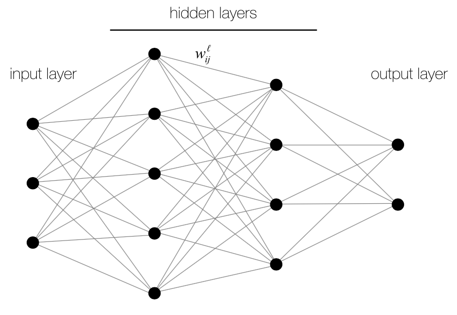 network has 2 hidden layers and is fully-connected.
A neuron in layer L receives inputs from all of the neurons in layer L – 1 with the input layer having no incoming connections. Each connection between 2 neurons i and j is associated with a weight wi,j which corresponds to the strength of the connection and can be negative or positive. The network is trained by presenting it with labeled training data in the form of m input-output pairs (x , y) = (x1 , y1) ... (xm , ym) where the x’s correspond to the activations of the input neurons and the y’s are the corresponding activations of the output neurons. The activation of neuron j in layer L is defined to be:
(1)
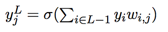
where σ(z) is a non-linear activation function, often taken to be the sigmoid
function, and yi is the activation of neuron i in the layer below.
The goal is to find the set of connection weights between each layer that produces the most accurate map between the inputs and outputs. The training is done by propagating inputs (xi) through the network to produce an output (y). This output is then compared to the desired output (yi) to calculate the value of the error function. The most commonly used error function is mean squared error (of all the output neurons) although others, such as cross-entropy, are also used (LeCun et al., 1998). The goal is then to change the weights in the network such that the cost function will be minimized and this is done via gradient descent and backpropagation. The standard weight update rule for backpropagation is:
(2) 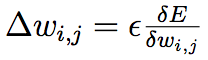
where ε is the learning rate and δE/δwi,j is the derivative of the error function with
respect to the weight (note that this depends on the error derivatives of all the neurons in deeper layers of the network).
The idea behind gradient descent is that because the error function is implicitly a function of the weights, the weights define an error surface and the goal is to find the minimum of this surface. The most efficient way to minimize error is to compute the gradient of the error function with respect to each weight and shift each weight in the opposite (because it is gradient descent not ascent) direction of its gradient (see (2)). This is easy to do for the output layer of neurons since it is their activations that are input into the error function. However, the weights of the hidden layers must also be updated in order to train the full network. This is done by defining error terms for each neuron (which implicitly depend on the activations of the output units) and using these to backpropagate error to each weight in the network. A derivation of the weight update rule can be found in [3]. Therefore, the degree to which a weight is changed is the product of the derivative of the error function with respect to that weight and a learning rate. The learning rate is usually a scalar factor that controls how far a weight is shifted. Networks with smaller learning rates generally take longer to learn but are more accurate and larger learning rates have the opposite effect.
While backpropagation is efficient at training feed-forward neural networks, which are loosely based on the computational architecture of the brain, there are several features of the algorithm that are biologically implausible or impossible. This is not surprising since the algorithm was not designed to be faithful to real neural circuits. However, the algorithm’s power to train networks to do complicated tasks and its relative simplicity to implement make it a very attractive model and beg the question of whether a similar process is being used in the brain. In this review, we will first outline the implausible features of backpropagation and several models that have attempted to make the algorithm more faithful to real neurons. We then examine other learning rules that achieve similar results through more biologically plausible means. We also look at properties and modifications of backpropagation that may allow it to solve the invariance problem in object recognition. Finally we examine the similarities between supervised and reinforcement learning and ask if reinforcement learning methods, of which there is extensive biological evidence, could achieve similar learning effects as the previously reviewed supervised methods.
Biologically implausible features of backpropagation
The first question that must be addressed is whether or not supervised learning, what backpropagation is used to do, even occurs in the brain? Addressing this, supervised motor learning appears to be extensive in the cerebellum (Koziol et al., 2014). It also seems to be responsible for the calibration of image stabilization on the retina and development of binocular vision in the frog Xenopus (Knudsen, 1994). In addition, at the end of this review, we review a model of area 7a parietal cortex, which combines features of supervised, and reinforcement learning. However, the extent to which supervised learning occurs elsewhere in the brain is not known.
One obvious difference between the ANNs on which backpropagation is used and biological neural networks is that the neurons of ANNs output real values while biological neurons output spikes (Bengio et al., 2016 arXiv unpublished). The argument could be made that biological neurons do output real values in the form of neurotransmitter. However, neurons release neurotransmitter in quantal packets (vesicles) meaning that they would only output discrete multiples of a base quantum not continuous real values (Liao et al, 1992). The real values output by model neurons in ANNs are typically interpreted to correspond to the firing rate of the neuron. However, it is very difficult for a real neuron to transmit its instantaneous firing rate making it necessary to sum the activity of a pool of neurons to estimate firing rate (Bohte et al., 2000). Furthermore, networks of spiking neurons have been proven to be able to do all of the computations that sigmoidal neurons are capable of (Maass, 1997). Bohte et al. have successfully adapted the backpropagation algorithm for a network of spiking neurons (termed SpikeProp), which was able to learn to solve the XOR problem, a classic test of non- linear classification. The model takes into account the internal state (voltage) of all of the neurons and uses a spike-response function to determine the postsynaptic voltage change in response to a presynaptic spike. In SpikeProp, output neurons
learn to predict spike times instead of real values. This model also uses mean squared error (differences in desired and actual spike times) as the error function and derives weight change rules very similar to normal backpropagation. Therefore, backpropagation can be adapted to train networks of spiking neurons.
Another biologically questionable feature of both backpropagation and SpikeProp is that error signals are propagated backwards by a different mechanism than the forward activation propagation. This is because each neuron requires knowledge of the activations (and output nonlinearities) of all of the neurons in deeper layers of the network in order to calculate the appropriate weight adjustment. This property of backpropagation is known as non-locality (O’Reilly, 1996). Hinton & McClelland (1987) were the first to try to address this issue and did so by proposing the “recirculation” learning procedure. Their model system had only 2 layers, a visible and a hidden layer where the visible layer represented both the input and output. This network was designed to output the same pattern as was input (the goal is to have the activations of the visible layer change as little as possible) while forcing the hidden layer to learn some interesting encoding of the input. This type of network is known as an auto-encoder (O’Reilly, 1996). The recirculation procedure works by propagating activity back and forth between the visible and hidden layer twice and calculating the error as the difference in the activation of the visible units between successive time steps (Fig. 2). Crucially, the weight update rule, which is very simple, only depends on local activation variables and does not require information about the output nonlinearities of the hidden units (Hinton & McClelland, 1987). The authors show that under some strong assumptions (linear visible units, symmetric weights between the 2 layers, and the use of regression to control the change in activation of both layers) this procedure closely approximates the gradient descent of normal backpropagation. While the use of exclusively local activation variables for weight adjustment is more biologically realistic, the assumptions necessary to make this system work well are not very realistic.
Therefore, supervised learning likely plays a role in the brain, backpropagation has been successfully adapted to spiking neurons, and gradient descent can be approximated using only local activation variables, although only under certain conditions. In the next section we will explore alternative learning rules including one in particular, GeneRec, which seems to unify what were previously thought to be quite different learning rules.
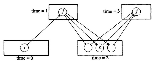
Figure 2. States of the visible (bottom) and hidden (top) units during the recirculation procedure. Time goes from left to right. (Taken from Hinton & McClelland, 1987).
Backpropagation as a member of a family of learning algorithms
There are many more biologically plausible models and learning rules in the literature (Mazzoni et al., 1991 ; Bogacz et al., 2000 are just a couple), however we will focus on just 4 in particular here because they have all been shown to be directly related to backpropagation. We have already discussed the recirculation algorithm and we will now discuss Almeida-Pineda (AP) backpropagation and contrastive-hebbian learning (CHL). We will end the section by discussing GeneRec, a learning algorithm from which both AP backpropagation and CHL can be derived as certain cases and which expands on the original recirculation algorithm.
AP backpropagation is an adaption of backpropagation to recurrent neural networks (Pineda, 1987 ; Almeida, 1990). This is a large step towards biological plausibility since there are extensive recurrent connections throughout the brain. Recurrent neural networks are different than feed-forward networks, and more difficult to train, because they can contain cycles and therefore require the activities of each neuron to be modulated in time. Therefore the activity of each neuron in the network is described by a differential equation and the network must settle into a steady state over time (Pineda, 1987). Therefore the outputs of a recurrent network are the steady state activations of the output neurons. While AP backpropagation extends backpropagation to recurrent networks, it still suffers from the problem of non-locality (O’Reilly, 1996).
The CHL learning algorithm is quite different from backpropagation. CHL was derived for recurrent networks (Boltzmann machines) and neurons in these networks use the same activation equation as in the AP formulation (O’Reilly, 1996). Weight changes in this algorithm are determined by the difference in activations of neurons between two different phases, the + phase and – phase (Hinton, 1989). In the + phase, the input neurons are clamped to the appropriate input activation and the output units are clamped to the corresponding output value. In the – phase, only the input values are clamped. At the end of the – phase, weights are updated according to the following rule:
(3) 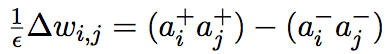
where ε is the learning rate, ai+ is the activation of presynaptic neuron i in the +
phase and aj+ is the activation of the postsynaptic neuron in the + phase (a- are activations of the same neurons in the – phase; O’Reilly 1996). Note that the weight change only depends on pre and postsynaptic activation variables. This is the key feature of CHL that makes it a biologically plausible learning algorithm.
O’Reilly (1996) presents a learning algorithm, GeneRec, which draws inspiration from the recirculation algorithm discussed earlier and shows that it is directly related to AP backpropagation and CHL. The GeneRec activation procedure is the same as in CHL, consisting of two phases where the input and output are presented together (+ phase) or the input is presented alone (- phase). O’Reilly uses a technical trick from the recirculation algorithm (which is based on approximations that are not proven to always hold but which empirical evidence indicates are reasonable) to derive the following learning rule for GeneRec:
(4) 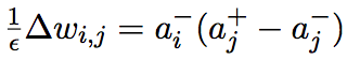
where the variables are the same as in (2). He then shows that under a few
constraints including symmetric recurrent weights and the technical trick of recirculation, this learning rule computes the same error derivatives as AP backpropagation. In addition, by modifying the learning rule to take into account the activation of neuron i (ai) in both the + and – phases as well as imposing reciprocal weight symmetry, GeneRec becomes identical to CHL (O’Reilly, 1996). It should be noted that weight symmetry is not imposed in the normal GeneRec algorithm. However, reciprocal weights seem to have a correspondence, which tends to make them symmetrical overtime nonetheless (O’Reilly, 1996). This is interesting since the weight symmetry improves the performance of GeneRec on several tasks and is important for calculating the correct error derivatives (O’Reilly, 1996). Based on the comparisons of the performance of AP backpropagation, CHL, and variations of GeneRec on various tasks, it is clear that without symmetric weights GeneRec does not learn nearly as well as AP backpropagation or CHL. Therefore, GeneRec is a general learning algorithm from which AP backpropagation and CHL can be approximated but without the constraint of symmetrical reciprocal weights it does not perform very well.
Backpropagation & the invariance problem
The problem of identifying percepts under various transformations (e.g. translation, scaling, and rotation for images or speed and frequency shifts for audio signals) is known as the “invariance problem”. This is something the human brain is able to do with ease but has not been able to be completely solved by automated systems. In this section we will discuss modifications to the backpropagation algorithm that make it more robust to variations of the input and will also discuss the use of predictive sparse decomposition (PSD) to have a network learn invariant features.
Demyanov et al. describe two separate modifications of the backpropagation algorithm that provide robustness against variations in the input (Demyanov et al., 2015). The first modification is dubbed Loss Invariant Backpropagation (Loss IBP) since it is designed to make the loss function more robust against all transformations of the input. This is done by adding an additional term to the loss function (and a second term to the weight update rule as a consequence), which uses information about the gradient of the loss function with respect to the input, which is calculated at the end of the backpropagation phase. This term is then minimized which results in local invariance to input transformations. This method requires an extra feed-forward pass through the network to propagate the new gradients and takes ~50% more time to train than standard backpropagation.
The second modification is termed Prediction IBP since it is designed to increase the robustness of the predictions of the network to input variation, not the loss the function (Demyanov et al., 2015). However, unlike Loss IBP, where the loss function is made robust against all variations, prediction IBP only trains the network to be robust to variations in the input along the direction of the gradient (gradient of the loss function w.r.t the input as in Loss IBP). It has been previously shown that modifying the input vector in the direction of the gradient of the loss function (i.e. in the direction that increases the error the most) generates what are known as adversarial examples, and that including these artificially generated examples in the training set improves performance (Goodfellow et al., 2015). Prediction IBP trains the network’s predictions to be more robust to variations of the inputs in the directions of these adversarial examples. This method is also very similar to a previous method, not discussed here, termed tangent backpropagation which allows a user to train their network to be robust to predetermined transformations (Simard et al., 2012). Through empirical testing, Prediction IBP was found to give better classification performance but at the cost of ~20% more training time (Demyanov et al., 2015). Therefore, both Loss IBP and prediction IBP allow for a network to become more robust to input variation and while prediction IBP allows for better performance, it requires more processing time.
We will now turn our attention to some interesting results from convolutional neural networks (CNNs) designed for object recognition, which have been pre-trained using PSD, an unsupervised learning method, to learn invariant features of the input. The primary advantage of deep neural networks and CNNs in particular is that these networks are capable of learning to build feature extractors, which before had to be arduously hand-engineered. CNNs are feed-forward neural networks with a structure loosely based on the primate visual cortex and have primarily been applied to image classification problems (LeCun, 2012). The basic unit of a CNN includes 4 components: a normalization layer (1), a convolution layer (2), a non-linear output layer (3), and a pooling layer (4) (LeCun, 2012). The convolution layer consists of a bank of learned linear filters that are convolved with the input to produce “feature maps” (LeCun, 2012). The non-linear output layer is the same as in standard neural nets where neurons output a non-linear function of their inputs. The pooling (sub sampling) layer is interesting in that it introduces some local invariance to input changes by smoothing the input-output relationships
of the layer below (LeCun, 2012). Therefore some invariance to local changes in input is obtained just from the structure of the CNN.
One method of learning invariant features of the input is to pre-train the filters of the convolution layers using an unsupervised learning algorithm (which will be fine tuned using supervised learning). LeCun notes that doing this has 2 primary advantages. The first is that it gives the network a favorable starting point before entering supervised learning and the second is that it allows the system to use large amounts of unlabeled data (LeCun, 2012). Predictive sparse decomposition is one such unsupervised learning algorithm, which uses an auto- encoder to learn sparse representations (sparseness is enforce via a penalty term in the loss function where more active units gets a higher penalty) of the inputs (LeCun, 2012). Learning the filters of the CNN using PSD results in filters that are very reminiscent of the receptive field properties of V1 cells (Figure 3; LeCun, 2012).
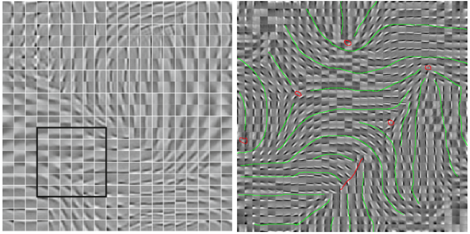
Figure 3. The filters that result from training with PSD show receptive properties very similar to cells in V1. (Taken from LeCun, 2012).
These filters represent the optimal features with which to encode the input images. Each filter is convolved with the input in the convolution layer, which gives translational invariance (LeCun, 2012). In addition, because filters of varying orientation and spatial frequency develop, the system has some invariance against rotation and scaling as well.
Therefore, while there are methods for increasing the robustness of backpropagation to input variations, the structure of the neural network itself can provide some robustness. Additionally, pre-training methods such as PSD can learn invariant feature sets from unlabeled data and produce results that compare very closely to that of the visual cortex.
Reinforcement Learning
Thus far we have been discussing problems in the realm of supervised learning, which require labeled input-output pairs to train a network. However, such training data is not always available. It may however, still be possible to “judge” the outputs of the network and provide feedback to the network in the form of a reward signal. This is the realm of reinforcement learning. The best example of reinforcement learning is action selection (Morita et al., 2016). In this problem, an animal does not know what action it should select so it uses a trial-and-error methodology to determine which actions result in a positive outcome. The learning occurs by using knowledge of the rewards of past actions to choose actions that will maximize future reward. There is extensive evidence of such learning occurring in the brain and it seems to be mediated by dopaminergic neurons that transmit a reward-prediction error signal (Shultz, 2016; Mazzoni et al., 1991; Morita et al., 2016; Kim et al., 2012; Fee & Goldberd, 2011). Dopamine has also been implicated in the induction of LTP further suggesting its role in learning (Lisman et al., 2011). So, there is strong evidence for reinforcement learning in the brain but how does this learning procedure differ from supervised learning and backpropagation?
Pure reinforcement learning, where there are no training examples, is simply not as powerful as supervised learning because the learner has access to less information (Barto et al., 2004). Reinforcement learning is a sequential search for actions that maximize reward, where each action is determined by the results of previous actions, while supervised learning involves mapping inputs to known outputs. Interestingly, any supervised learning problem can be converted to a reinforcement-learning problem by making the loss function such that high error corresponds to low reward and low error high reward. However, you cannot convert a strictly reinforcement learning problem into a supervised learning problem. Barto et al. note that if you already have a set of action-reward pairs (a list of previous actions and their corresponding rewards), then you can approximate the reward function via standard supervised learning and use this to guide future action selection. It is likely then, that the brain uses a combination of ideas from reinforcement learning and supervised learning such as in the model described below.
Mazzoni et al. describe a method for training a model of area 7a parietal cortex, which is thought to compute head-centered coordinates, which only uses a global reward signal (Mazzoni et al., 1991). In this method, an input is presented to a feed-forward network and propagated to the output layer. The reward signal is calculated by comparing the activations of the output units to desired values and is propagated back to the network via feedback connections. Because desired values are specified, this is technically a supervised learning algorithm. However, unlike normal backpropagation where each unit in the network adjusts its weights according to a unique error derivative, each unit in this network receives the same scalar reward value. Each unit then updates its weights as a function of this scalar reward, its excitability (probability of firing), and pre/post synaptic activations, all of which are local variables. The network was trained to perform the task to any level of accuracy (Mazzoni et al., 1991). However, because each unit receives the
same reward value instead of a unique error gradient, the learning of the system is much noisier (it only approximates the exact error gradients calculated by backpropagation). Therefore this model has many attractive qualities such as the ability to train a network using only local activation variables and a global reward signal, which aligns it with the evidence for Hebbian plasticity as well as dopamine’s role in synaptic plasticity. The downside of the method is that learning is noisier, although this is expected in biological learning, and it is not as powerful as standard backpropagation (O’Reilly, 1996; Xie & Seung, 2003). Additionally, this method does not actually employ strict reinforcement learning because it calculates reward via known desired output values. However these values may be internally generated, as they are thought to be in birdsong (Fee & Goldberg, 2011), which would bring this model closer to other reinforcement literature.
In this section we have compared the distinct problems of reinforcement and supervised learning and concluded that supervised learning is more powerful because it is able to make use of more data. However, there is undeniable evidence of reinforcement learning principles at work in the brain. We then reviewed a learning procedure that uses elements of both supervised and reinforcement learning and approximates the results of backpropagation.
Conclusion
Our aim in this review is to assess the biological plausibility of the backpropagation algorithm and to examine its relationship to other proposed learning rules. We reviewed models that extended the backpropagation algorithm to spiking neural networks (SpikeProp) as well as recurrent networks (AP backpropagation). We also looked at models that approximate backpropagation using only local activation variables (recirculation, GeneRec). We addressed how backpropagation alone, and in conjunction with certain network architectures can be used to help solve the invariance problem, which is a key ability of biological systems. Finally, we examined the relationship between supervised learning and reinforcement learning, determining that supervised learning is more efficient but requires labeled data and suggesting that a combination of both is likely at play in the brain. We end by reviewing a model that combines aspects of both learning modalities to approximate the learning of backpropagation. All of this suggests that actual backpropagation is probably not occurring in the brain but that there are alternative, more biologically plausible, learning methods that achieve similar performance and are likely important for all aspects of learning and memory.
Works Cited
Henry J. Kelley (1960). Gradient theory of optimal flight paths. Ars Journal, 30(10), 947-954.
Yann LeCun, L. B., Genevieve B. Orr, and Klaus-Robert Muller (1998). "Efficient BackProp." Neural Neworks: tricks of the trade.
Rumelhart, D. E., et al. (1986). "Learning representations by back- propagating errors." Nature 323(6088): 533-536.
Koziol, L. F., et al. (2014). "Consensus Paper: The Cerebellum's Role in Movement and Cognition." The Cerebellum 13(1): 151-177.
Yoshua Bengio, D.-H. L., Jorg Bornschein, Thomas Mesnard and Zhouhan Lin (2016). "Towards Biologically Plausible Deep Learning." arXiv.
Liao, D., et al. (1992). "Direct measurement of quantal changes underlying long-term potentiation in CA1 hippocampus." Neuron 9(6): 1089-1097.
Bohte, S. M., et al. (2000). Error-backpropagation in temporally encoded networks of spiking neurons, CWI (Centre for Mathematics and Computer Science).
Maass, W. (1997). "Fast Sigmoidal Networks via Spiking Neurons." Neural Computation 9(2): 279-304.
O’Reilly, R. C. (1996). "Biologically Plausible Error-Driven Learning Using Local Activation Differences: The Generalized Recirculation Algorithm." Neural Computation 8(5): 895-938.
Hinton, G. E. and J. L. McClelland (1987). Learning representations by recirculation. Proceedings of the 1987 International Conference on Neural Information Processing Systems, MIT Press: 358-366.
Mazzoni, P., et al. (1991). "A more biologically plausible learning rule for neural networks." Proc Natl Acad Sci U S A 88(10): 4433-4437.
Bogacz, R., et al. (2000). Frequency-based error backpropagation in a cortical network. Neural Networks, 2000. IJCNN 2000, Proceedings of the IEEE-INNS- ENNS International Joint Conference on.
Pineda, F. J. (1987). "Generalization of back-propagation to recurrent neural networks." Physical Review Letters 59(19): 2229-2232.
Almeida, L. B. (1990). A learning rule for asynchronous perceptrons with feedback in a combinatorial environment. Artificial neural networks. D. Joachim, IEEE Press: 102-111.
Hinton, G. E. (1989). "Deterministic Boltzmann learning performs steepest descent in weight-space." Neural Comput. 1(1): 143-150.
Demyanov, S. B., James; Kotagiri, Ramamohanarao; Leckie, Christopher (2015). Invariant backpropagation: how to train a transformation-invariant neural network. Internatinal Conference on Learning Representations, ARXIV.
Goodfellow, I. J. S., Jonathon; Szegedy, Christian (2015). Explaining and Harnessing Adversarial Examples. ICLR.
Simard, P. Y., et al. (2012). Transformation Invariance in Pattern Recognition – Tangent Distance and Tangent Propagation. Neural Networks: Tricks of the Trade: Second Edition. G. Montavon, G. B. Orr and K.-R. Müller. Berlin, Heidelberg, Springer Berlin Heidelberg: 235-269.
LeCun, Y. (2012). Learning invariant feature hierarchies. Proceedings of the 12th international conference on Computer Vision - Volume Part I. Florence, Italy, Springer-Verlag: 496-505.
Morita, K., et al. (2016). "Corticostriatal circuit mechanisms of value-based action selection: Implementation of reinforcement learning algorithms and beyond." Behav Brain Res 311: 110-121.
Schultz, W. (2016). "Dopamine reward prediction-error signalling: a two-
component response." Nat Rev Neurosci 17(3): 183-195. 22.Fee, M. S. and J. H. Goldberg (2011). "A hypothesis for basal ganglia- dependent reinforcement learning in the songbird." Neuroscience 198: 152- 170.
Lisman, J., et al. (2011). "A neoHebbian framework for episodic memory; role of dopamine-dependent late LTP." Trends Neurosci 34(10): 536-547.
Barto, A. G., et al. (2004). Reinforcement Learning and Its Relationship to Supervised Learning. Handbook of Learning and Approximate Dynamic Programming, John Wiley & Sons, Inc.: 45-63.
Xie, X. and H. S. Seung (2003). "Equivalence of backpropagation and contrastive Hebbian learning in a layered network." Neural Comput 15(2): 441-454.