Cellular Automata via Excel

Cellular automata are an important computational and modeling tool in studying highly complex, nonlinear phenomena. While they were first formalized in the 1940s by John von Neumann (as an alternative computational model to the famous Turing machine described by Alan Turing), their prolific use can be dated to the much more recent work of Stephen Wolfram - the creator of the Mathematica programming language and Wolfram Alpha platform, particularly to his book A New Kind of Science , published in 2002.

In this post we will be exploring a very simple kind of cellular automaton, an elementary cellular automaton which consists of a single row of cells (as opposed to a grid of cells, which is the typical setup of a cellular automaton). Surprisingly, even this simple "elementary" automaton can do a lot - as we will see in due course.

So, what is a cellular automaton? In a nutshell it is a collection of simple single-purpose computation units (called cells) that "compute" their next state (aka configuration) based only on "local" information, their private, local state - the state of their neighbors. This last part sets them apart from Turing machines which can and do refer to the global state.

This concept of locality - the cell's "neighborhood" is crucial in grasping how cellular automata work. In the case of a 1-dimensional elementary cellular automaton (a single row of cells), the neighborhood of a cell is comprised of 3 cells - the cell itself and the immediate adjacent cells to the left and to the right. If we think of a 2-D cellular automaton (a grid of cells), we have up to 9 neighbors - 3 above, 3 below and 3 on the same level (see pic.0). Can you think of how many neighbors a 3-D cellular automata could have?

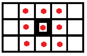
Pic. 0

The cellular automaton model of computation has some profound advantages over the Turning model because calculations can be done in a massively parallel fashion - all the cells can be computing their state all at once, because they do not rely on or change shared global information. With the rise of multi-core PCs this computational paradigm is becoming increasingly dominant. Incidentally, this is exactly how biological systems and other real life systems function - brains, electrical pathways, spread of contagious diseases, population growth, etc. Thus, it makes sense to use computation methods that mimic the phenomena themselves.

Enough theory, let's look at an example!

Pic. 1

What we see here is an elementary 1-dimensional 9-cell CA (that's the abbreviation we'll be using from now on for cellular automaton) with a certain state (configuration ) at time 1. What happens at time =2 ? Well, that depends on the "rules" that govern a given CA. A particular rule that we will be implementing in Excel is called "rule 184" and it is described as follows:

current pattern	111	110	101	100	011	010	001	000
new state for center cell	1	0	1	1	1	0	0	0

So, how does this work? Let's look at current pattern "110" (the highlighted one). What this rule is saying is that if the cell's current state is 1 and it's left neighbor's state is also 1, but it's left neighbor's state is 0, then its next state will be 0. See if you can apply this rule to the sample CA (pic.1), omitting the leftmost and rightmost cells (we will deal with them in a moment).

Did you get something like this (pic.2)?

Pic.2

As you can see, we have omitted the rightmost and leftmost cells because it is not immediately clear where we get the values of their left and right neighboring cells - since they are located on the edges. There are several options. One is to consider the CA as wrapping around on itself, in which case the rightmost cell's right neighbor is the leftmost cell and the leftmost cell's right neighbor is the rightmost cell. Another option is to use the value of "0" for missing cells. Finally, one can apply a special rule for those cells. We will go with the first option because it actually models our real-life phenomenon more accurately. Thus, you could think of the CA as a cylinder with no edges.

Thus, the value of the leftmost cell comes from configuration 000 resulting in 0, and the rightmost 100, resulting in 1. The final result is shown below (pic.3):

Pic.3

OK, so hopefully this intro was sufficient to get the basic ideas across; now let's build something useful. We are going to be using "Rule 184" because it is actually based on a real-life phenomenon of streaming motion, particularly applicable to things like traffic. What we want to model is a junction that allows cars to enter an circular lane with 13 exit points such that we minimize possible jams. We want to figure out a dynamic "stop" light that will allow maximum cars to enter the circular lane with minimum number of possible jams. In order to do that we will assume that all the cars will only use the last exit, thus creating the worst possible scenario. Amazingly, this elementary CA that uses Rule 184 will allow us to successfully solve this rather tricky problem.

So, let's fire up Excel and get to work! (Place the cursor in each cell mentioned in the beginning of the instruction, follow the instructions and then press Enter at the end).

A1 - type in "Bitmask values", ALT-Enter , "(powers of 2)".
B1 - type in "1"
C1 - type in "=", select B1 and type "*2"
Use the mouse to select the lower right hand cross-hair of C1 and drag it across to N1.

You should now have a series ranging from 1 to 4096. We are going to use this top row to assign a numeric value to each CA configuration, as well as load our initial configuration, using something called a bitmask. Bitmasks are super easy as we'll see in a minute. (If you are savvy at math you have already figured out that this simple trick allows us to enumerate up to 2^13 or 2*4096-1 configurations. Not bad!) Anyway, let's keep going.

A2 - type in "=RANDBETWEEN(0,N1*2-1)"
A3 - type in "Initial state bitmask"
B3 - type in "=IF(BITAND(B1,$A$2)=B1,1,0)"
Use the mouse to select the lower right hand cross-hair of B3 and drag it across to N3

OK, so what have we gotten here? The RANDBETWEEN function will give us a new random value for our trial runs - a way to simulate random traffic condition. What we do next is translate that number into something our CA can understand - 0s and 1s. To do that we use BITAND function which takes a random number and "ANDs" it with a given power of 2 (producing a binary bitmask of the random number). If the result contains the number we are ANDing with, then we use IF function to output 1, otherwise - 0. You can get some intuition about how that works by just typing some numbers in cell A2. If you type any number that's a power of 2, like say 64, your bitmask will be all zeroes except for the column that corresponds to 64. If you type 69, columns B, D and H will have 1s, while all the others will be zeroes (because 69 = 1+4+64).

In short, what we have gotten so far is the initial state for our CA to operate on in succession. Now, we are going to actually encode the "Rule 184" and get the show on the road!

But, first let's add a bit of formatting to make the model a bit more visually intuitive.

Right-click on row 1 and click on "Hide" - we don't really need to see it once it's set up
Select A2 and A3 and use Excel's Input automatic highlighting to show that these are inputs into the formula and are in fact related
Select B3 through N3. Click on "Conditional Formatting" and select "Manage Rules". (pic 4)

Pic.4

Click on "New Rule"
Select a rule type of "Format only cells that contain"
Set the options to "Cell value", "equals to", "0"
Click on "Format" and choose some greenish color (0 means that the spot is empty, so it's not jammed)

Repeat the steps above only choose "1" for value and some reddish color for cells that are jammed.
Click "OK".

If you want to add additional pizzazz, add a rule of type "Format all cells based on their values", in the format styles drop-down select "Icons sets" and set the options as pictured below (pic. 5):

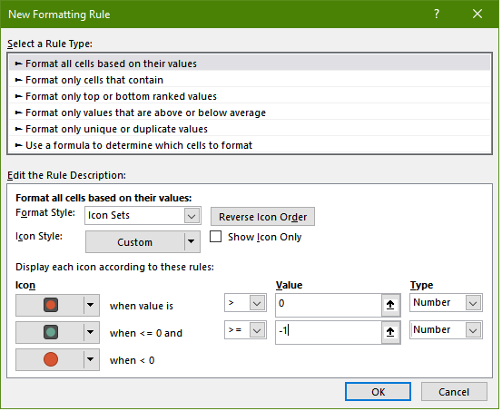
Pic. 5

Click "OK". This will add cool little traffic lights to your model.

Well, that was fun, but let's get back to our CA and implementing rule 184.

C4 (this should be right below the second leftmost cell containing the first bit of the original configuration) - type in "=IF(OR(AND(B3=1,C3=1,D3=1),AND(B3=1,C3=0,D3=1),AND(B3=1,C3=0,D3=0),AND(B3=0,C3=1,D3=1)),1,0)"
Select the cross hairs of cell C4 and drag it to M4 (notice we are omitting the edge cells because the logic has to be a little different to accommodate the same rule).

This formula should make some intuitive sense - if we are in C4 , our previous state was in C3 and therefore our neighborhood is made up of B3, C3 and D3 - the values that our CA is examining. It is a good idea at this point to go back to the definition of rule 184 and do some quick spot checking to make sure our CA is working properly. Find a few patterns and make sure that the resulting computed value is correct.

After verifying that everything looks good, let's finish up with the edge cells.

B4 - type in "=IF(OR(AND(N3=1,B3=1,C3=1),AND(N3=1,B3=0,C3=1),AND(N3=1,B3=0,C3=0),AND(N3=0,B3=1,C3=1)),1,0)"
N4 - type in "=IF(OR(AND(M3=1,N3=1,B3=1),AND(M3=1,N3=0,B3=1),AND(M3=1,N3=0,B3=0),AND(M3=0,N3=1,B3=1)),1,0)"

Do you see what we are doing here? In the first case we use the last cell of the previous row as our leftmost neighbor and in the other case we use the first cell of the previous row as our rightmost neighbor. Does it make sense in light of our modeling of traffic flow? When you think about it, yes, it does - because the flow is continuous, just like a surface of a cylinder, and we expect the same pattern to surround us both in front and before us.

Now that we have our first CA computation let's copy it down so we can see how a lane will operate after N iterations. How many do you want to do? A 100? That's what I was thinking too :).

Select cells B4 through N4; use the mouse cursor to select the cross hairs of N4 and drag it down to N103
O4 - type in "iteration#". Press Ctrl+B to bold the contents.
O5 - type in "1"
O6 - type in "=O5+1". Select the cross hairs of O6 and double-click - this will propagate the formula down to row 103. We now have 100 iterations of CA model. Highlight cells O4-O103 and use light yellow color to format them differently from the CA cells.
Place cursor in B1. Click on the "Format Painter" brush and select all the CA cells - the range B4:O103. Your screen should looks something like the following (pic. 6)

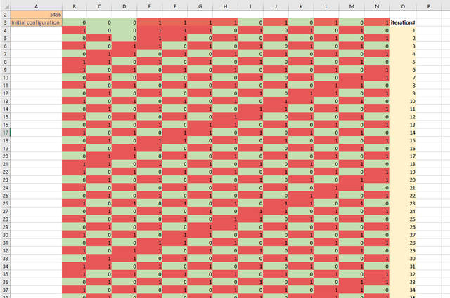
Pic. 6

Obviously, the number in A2 is random, so it will be different from the one you see here. You can press F9 repeatedly to see how the screen changes with a different configuration.

OK, so what's next? Well, now we want to have some way to quantify the effectiveness of each configuration. To do that we will introduce two metrics - the # of cars (throughput) and the number of car jams. For each row in CA the number of cars is simply the number of cells with a value of 1. The number of car jams will be the number of adjacent 1's. We also want to keep track of how configurations change - their periodicity. This is important, because we want to favor a stable configuration that tends to return quickly to its starting point. Something that's highly unpredictable will have a period approaching the total # of possible configurations (8191 in this case) and that is not very desirable.

Let's go to work!

P3 - type in "Traffic jams"
Q3 - type in "Throughput"
R3 - type in "Configuration"
P4 type in "=SUM(BITAND(B4,C4),BITAND(C4,D4),BITAND(D4,E4),BITAND(E4,F4),BITAND(F4,G4),BITAND(G4,H4),BITAND(H4,I4),BITAND(J4,K4),BITAND(K4,L4),BITAND(L4,M4),BITAND(M4,N4))"

Q4 type in "=COUNTIF(B4:N4,"=1")"
R4 type in "=SUMPRODUCT($B$1:$N$1,B4:N4)"
Select cells P4 through R4 and double click on the cross hairs of R4. This should copy the formulas down to row 103.
P105 - on the Home tab of Excel click on Auto-Sum and select "sum". It should sum up cells P4:P104
Q106- similarly, click on Auto-Sum and select "sum". It should sum up cells Q4:Q105
B105 - type in "Total jams". Select cells B105:P105 and add a thin bottom border.
B106 - type in "Total througput (cars)". Select cells B106:Q106 and add a thin bottom border.

What is going on here? We are using BITAND function again to see if two adjacent cells have 1's in them; if they do - BITAND returns 1, otherwise it returns 0. Summing all the results gives us the total # of car jams. Throughput is even easier - we use COUNTIF to count all the cells that have 1 in them.

R4 essentially converts the binary bitmask of each row to a decimal number by multiplying the hidden row of powers of two by the corresponding 0 or 1.

Now let's add a visualization of our model.

Select cells P3:R103. Click on Insert tab in Excel menu. Select "Line Chart" and "Line Chart with Markers" in the submenu. You will notice that the configuration line obscures the traffic jams and throughput lines, so we'll graph it on a separately scaled axis. Double click on the line representing the configuration. You should see something similar to the screenshot below (pic. 7).

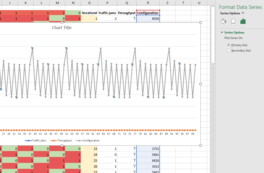
Pic.7

Select "Secondary axis". Format the line so it uses a different dash type and has smaller thickness.

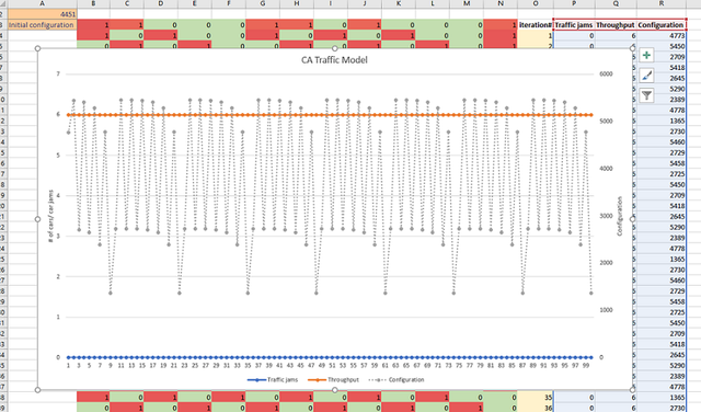
Add axis titles - "# of cars/car jams" to the primary vertical axis and "config #" to the secondary vertical axis. (You can do this by double-clicking on the graph and then selecting a menu from the "Add Chart Element" in the top left corner of Excel window). Change graph title to "CA Traffic Model". Your graph should resemble pic.8 below.

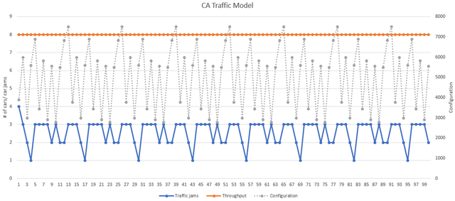
Pic.8

Press F9 repeatedly to see how the graph changes with a different starting configuration. Do you see data that's more or less periodic?

Well, I guess we could just stop here and let you press F9 while keeping an eye on the total # of cars that passed through vs. total number of jams - until your fingers would go completely numb. Thankfully, there is a better way to find an optimal solution. First we need to quantify our fitness function - something that converts our intuition that we want to maximize benefit/cost ratio of throughput to car jams. Let's do that first.

B107 - type in "Fitness function"
R107 - type in "=Q106-POWER(P105,1.5)"
B108 - type in "Trial Value"
C108- type in 0
A2 - change the formula to "=FLOOR.MATH(C108)"

We are going to use C108 as our input to Excel Solver. The solver uses continuous values and we need to convert them to discrete integers - hence our change to A2's formula.

To activate Solver click on "File - Options - Add-ins". Find "Solver Add-in" - it will most likely be listed in the "Inactive Application Add-ins" category. Click on "Go" next to "Manage Excel Add-ins". Check the box that says "Solver" and click "OK". (see pic.9)

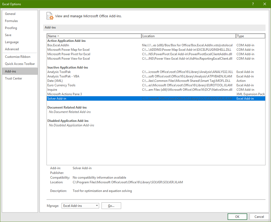
Pic.9

If everything worked you should now have "Solver" icon inside "Analyze" section on the Data tab of Excel. Click on it. (see pic.10).

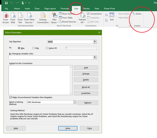
Pic.10

Notice that you have something called "Set Objective". Select cell R107 (that contains our fitness function) and leave "Max" as the default. In "By changing variable cells" select C108 - the input we will be changing. Now we need to add 2 constraints - the lower and upper bound. The lower bound will be 0, the upper bound 8191 - our maximum bitmask configuration (remember our CA is only 13 cells wide, so it can only support 2^13-1 combinations). Select solving method of "Evolutionary".

Your dialogue box should look like the one shown below (pic.11).

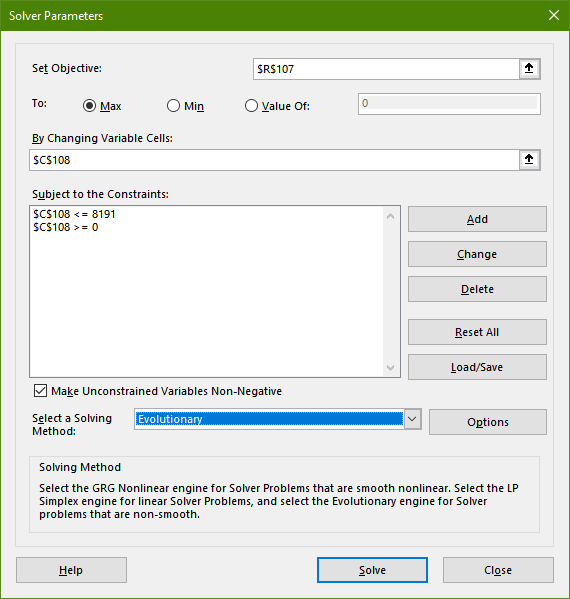
Pic.11

Now, click on "Solve" and go have some coffee (this could take several minutes depending on how fast your PC is)! If the Solve is working, you will see in Excel status bar something like "Setting up problem.... Incumbent solutions... subproblem... trial run....".

Anyway, after a few minutes you should get a solution. The one I got was with 600 car throughput and 0 jams - given by the initial configuration of 4451. (keep in mind there could be a number of optimal solutions to these highly nonlinear problems). What did you get?

Look at your graph - how does periodicity look? Is this a stable or a rather chaotic pattern? Congratulations, you just helped traffic control find an optimal traffic light pattern that maximizes car flow!