Coding Neural Network Back-Propagation Using C# part 2

Vote. and the second part will be released. the source in the last part.
var example = true
Training using back-propagation is accomplished with these statements:

Console.WriteLine("Starting training");
double[] weights = nn.Train(trainData, maxEpochs,
  learnRate, momentum);
Console.WriteLine("Done");
Console.WriteLine("Final weights and biases: ");
ShowVector(weights, 2, 10, true);

The Train method stores the best weights and bias values found internally in the NeuralNetwork object, and also returns those values, serialized into a single result array. In a production environment you would likely save the model weights and bias values to a text file so they could be retrieved later, if necessary.
The demo program concludes by calculating the prediction accuracy of the neural network model:

  double trainAcc = nn.Accuracy(trainData);
  Console.WriteLine("Final accuracy on train data = " +
    trainAcc.ToString("F4"));
  double testAcc = nn.Accuracy(testData);
  Console.WriteLine("Final accuracy on test data = " +
    testAcc.ToString("F4"));
  Console.WriteLine("End back-propagation demo");
  Console.ReadLine();
} // Main

The accuracy of the model on the test data gives you a very rough estimate of how accurate the model will be when presented with new data that has unknown output values. The accuracy of the model on the training data is useful to determine if model over-fitting has occurred. If the prediction accuracy of the model on the training data is significantly greater than the accuracy on the test data, then there's a strong likelihood that over-fitting has occurred and re-training with new parameter values is necessary.
Implementing Back-Propagation Training
In many areas of computer science, Wikipedia articles have become de facto standard references. This is somewhat true for the neural network back-propagation algorithm. A major hurdle for many software engineers when trying to understand back-propagation, is the Greek alphabet soup of symbols used. Figure 2 presents 11 major symbols used in the Wikipedia explanation of back-propagation. Bear with me here; back-propagation is a complex algorithm but once you see the code implementation, understanding these symbols isn't quite as difficult as it might first appear.

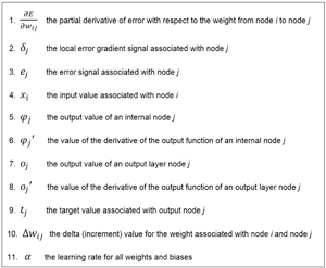
[Click on image for larger view.] Figure 2. Symbols Used in the Back-Propagation Algorithm
The definition of the back-propagation training method begins by allocating space for gradient values:

public double[] Train(double[][] trainData,
  int maxEpochs, double learnRate, double momentum)
{
  double[][] hoGrads = MakeMatrix(numHidden,
    numOutput, 0.0); // hidden-to-output weight gradients
  double[] obGrads = new double[numOutput];
  double[][] ihGrads = MakeMatrix(numInput,
    numHidden, 0.0);  // input-to-hidden weight gradients
  double[] hbGrads = new double[numHidden];
...

Back-propagation is based on calculus partial derivatives. Each weight and bias value has an associated partial derivative. You can think of a partial derivative as a value that contains information about how much, and in what direction, a weight value must be adjusted to reduce error. The collection of all partial derivatives is called a gradient. However, for simplicity, each partial derivative is commonly just called a gradient.
The key math equations of back-propagation are presented in Figure 3. These equations can be intimidating. But interestingly, even for my colleagues who are math guys, many feel that the actual code is easier to understand than the equations.

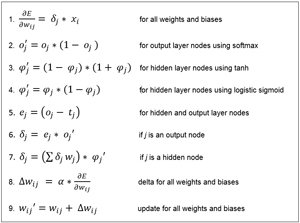
[Click on image for larger view.] Figure 31. The Key Equations for Back-Propagation
If you look at the equations in Figure 3 (and your head doesn't explode), you'll see that the weight update (equation 9) is the goal. It involves a weight delta (symbol 10). Calculating the delta (equation 8) uses the learning rate (symbol 11) and the gradients (symbol 1). In code, the values of each of these gradients are stored in hoGrads (hidden-to-output weights), obGrads (output biases), ioGrads (input-to-hidden weights), and hbGrads (hidden biases).
Next, storage arrays for the output and hidden layer local error gradient signals (symbol 2) are allocated:

double[] oSignals = new double[numOutput];
double[] hSignals = new double[numHidden];

Unlike most of the other variables in back-propagation, this variable doesn't seem to have a consistently used standard name, and Wikipedia uses the symbol, which is lowercase Greek delta, without explicitly naming it. I call it the local error gradient signal, or just signal. Note, however, that the similar terms "error signal" and "gradient" have different uses and meanings in back-propagation.

The momentum term is optional, but it is almost always used with back-propagation. Momentum requires the values of the weight and bias deltas (symbol 10) from the previous training iteration. Storage for these previous iteration delta values is allocated like so:

double[][] ihPrevWeightsDelta = MakeMatrix(numInput,
  numHidden, 0.0);
double[] hPrevBiasesDelta = new double[numHidden];
double[][] hoPrevWeightsDelta = MakeMatrix(numHidden,
  numOutput, 0.0);
double[] oPrevBiasesDelta = new double[numOutput];

The main training loop is prepared with these statements:

int epoch = 0;
double[] xValues = new double[numInput];
double[] tValues = new double[numOutput];
double derivative = 0.0;
double errorSignal = 0.0;
int errInterval = maxEpochs / 10;

Variable epoch is the loop counter variable. Array xValues holds the input values from the training data. Array tValues holds the target values from the training data. Variable derivative corresponds to symbols 6 and 8 in Figure 2. Variable errorSignal corresponds to symbol 3. Variable errInterval controls how often to compute and display the current error during training. Before the training loop starts, an array that holds the indices of the training data is created:

int[] sequence = new int[trainData.Length];
for (int i = 0; i < sequence.Length; ++i)
  sequence[i] = i;

During training, it's important to present the training data in a different, random order each time through the training loop. The sequence array will be shuffled and used to determine the order in which training items will be processed. Next, method Train begins the main training loop:

while (epoch < maxEpochs)
{
  ++epoch;
  if (epoch % errInterval == 0 && epoch < maxEpochs)
  {
    double trainErr = Error(trainData);
    Console.WriteLine("epoch = " + epoch +
      " error = " + trainErr.ToString("F4"));
  }
  Shuffle(sequence);
...

Calculating the mean squared error is an expensive operation because all training items must be used in the computation. However, there's a lot that can go wrong during training so it's highly advisable to monitor error. Helper method Shuffle scrambles the indices stored in the sequence array using the Fisher-Yates algorithm. Next, each training item is processed:

for (int ii = 0; ii < trainData.Length; ++ii)
{
  int idx = sequence[ii];
  Array.Copy(trainData[idx], xValues, numInput);
  Array.Copy(trainData[idx], numInput, tValues,
    0, numOutput);
  ComputeOutputs(xValues); 
...

The input and target values are pulled from the current training item. The input values are fed to method ComputeOutputs, which does just that, storing the output values internally. Note that the explicit return value array from ComputeOutputs is ignored. Next, the output node signals (equation 6) are computed:

for (int k = 0; k < numOutput; ++k)
{
  errorSignal = tValues[k] - outputs[k];
  derivative = (1 - outputs[k]) * outputs[k];
  oSignals[k] = errorSignal * derivative;
}

The error signal (equation 5) can be computed as either output minus target, or target minus output. The Wikipedia article uses output minus target which results in the weight deltas being subtracted from current weight values. Most other references prefer the target minus output version, which results in weight deltas being added to current weight values (as shown in equation 9).
The Wikipedia entry glosses over the fact that the output derivative term depends on what activation function is used. Here, the derivative is computed assuming that output layer nodes use softmax activation, which is a form of the logistic sigmoid function. In the unlikely situation that you use a different activation function, you'd have to change this part of the code.
After the output node signals have been computed, they are used to compute the hidden-to-output weight and output bias gradients:

for (int j = 0; j < numHidden; ++j)
  for (int k = 0; k < numOutput; ++k)
    hoGrads[j][k] = oSignals[k] * hOutputs[j];
 
for (int k = 0; k < numOutput; ++k)
  obGrads[k] = oSignals[k] * 1.0;

Notice the dummy 1.0 input value associated with the output bias gradients. This was used just to illustrate the similarity between hidden-to-output weights, where the associated input value comes from hidden layer node local output values, and output node biases, which have a dummy, constant, input value of 1.0. Next, the hidden node signals are calculated:

for (int j = 0; j < numHidden; ++j)
{
  derivative = (1 + hOutputs[j]) * (1 - hOutputs[j]); //tanh
  double sum = 0.0; 
  for (int k = 0; k < numOutput; ++k) {
    sum += oSignals[k] * hoWeights[j][k]; 
  }
  hSignals[j] = derivative * sum; 
}

These calculations implement equation 7 and are the heart of the back-propagation algorithm. They're not at all obvious. The Wikipedia entry explains the beautiful, but complicated math, which gives equation 7. The Wikipedia entry assumes the logistic sigmoid function is used for hidden layer node activation. I much prefer using the hyperbolic tangent function (tanh) and the value of the derivative variable corresponds to tanh. Notice the calculations of the hidden node signals require the values of the output node signals, essentially working backward. This is why back-propagation is named what it is.